Copyright © 1992 by Annual Reviews. All rights reserved
| Annu. Rev. Astron. Astrophys. 1992. 30:
429-456 Copyright © 1992 by Annual Reviews. All rights reserved |


Once the Galaxy is removed, the XRB shows a large-scale anisotropy which
is consistent with the dipole expected from our motion with respect to
the MWB
(Shafer 1983,
Shafer & Fabian 1983,
Boldt 1987).
One major
difference with the MWB, is that source confusion dominates over the
expected dipole (which corresponds to
 I/I = (3 +
  )v/c = 0.5%, where v is
our velocity relative to the MWB and the spectral index
= 0.4) on any
angular scale less than about 90. It is then a very difficult task to
detect this systematic effect and the uncertainties involved are high.
)v/c = 0.5%, where v is
our velocity relative to the MWB and the spectral index
= 0.4) on any
angular scale less than about 90. It is then a very difficult task to
detect this systematic effect and the uncertainties involved are high.
In the 2-10 keV band, the direction inferred for the XRB dipole (l =
280°, b = 30°) is consistent (within the 1 or
2 error contours) with
the MWB dipole. The inferred velocity is 475 ± 165 km
s-1, roughly
consistent with the expected ~ 360 km s-1, but still allowing
for some of
the effect to be caused by an enhancement of the local X-ray emissivity
towards this direction
(Miyaji & Boldt 1990).
At higher energies (80-165
keV) a dipole fit to the X-ray intensity distribution gives I =
300° and
b = 30° with a velocity 960 ± 520 km s-1
(Boldt 1987,
Gruber 1992),
which is consistent with the A2 data.
error contours) with
the MWB dipole. The inferred velocity is 475 ± 165 km
s-1, roughly
consistent with the expected ~ 360 km s-1, but still allowing
for some of
the effect to be caused by an enhancement of the local X-ray emissivity
towards this direction
(Miyaji & Boldt 1990).
At higher energies (80-165
keV) a dipole fit to the X-ray intensity distribution gives I =
300° and
b = 30° with a velocity 960 ± 520 km s-1
(Boldt 1987,
Gruber 1992),
which is consistent with the A2 data.
Other large-scale features are now being seen with a careful inspection of HEAO-1 and even Ariel V data. Some voids and superclusters seen in optical catalogues coincide with cold and hot spots in the XRB (Jahoda & Mushotzky 1989, Mushotzky 1992; Figure 2). An interesting result is also emerging from work by Jahoda et al (1991), in which fluctuations in the HEAO-1 data are cross-correlated with optical counts of bright galaxies. A significant correlation [of amplitude (3 ± 1) x 10-3] is found, probably due to nearby sources just unresolved by the HEAO-1 A2 instrument (mostly AGN) which lie in regions of higher than average galaxy density. The correlation may be related to the void and supercluster effect. (Note that at least a few percent of the XRB originates at low z from unresolved sources. Large variations in this component then lead to detectable spatial fluctuations in the intensity of the XRB.)
Intrinsic sky fluctuations are always detected on small angular scales when instrumental noise such as that due to photon counting is small enough. These fluctuations are due to those sources which are just not resolved by the detector beam. Following earlier work on the radio sky (Scheuer 1957), they can be modeled as ``P(D) noise'' (see e.g. Scheuer 1974, Fabian 1975, Warwick & Stewart 1989, Hayashida 1990, Barcons & Fabian 1990) which is the distribution of fluctuations (i.e. deviations from the mean, or deflections D in early radio parlance) in the integrated flux from sources present in different pointing directions. The P(D) curve is the histogram of all fluctuations for a given beam size. The positive tail of this distribution is dominated by the brightest sources just below the detection threshold. Very faint sources, of which there may be many per beam, only produce a further small quasi-Gaussian broadening to this distribution. The major contribution to the width of the P(D) distribution is due to the flux level at which there is about one source per beam. Fluctuations in the XRB can therefore be used to test the source counts (the log N-log S curve) down to this level. The faintest level that can be probed by this method depends on the level of instrumental and systematic noise and on the number of samples used.
The P(D) curve is always skewed due to the presence of the sources that are just not resolved. The positive tail dominates the low-order moments and in particular the variance. For most log N-log S curves the variance goes to infinity as the detection threshold (i.e. the level above which a source is claimed to have been found and therefore excluded from the background analysis) is increased. It is then inappropriate to use just the second moment to describe the P(D) curve instead of fitting the whole distribution.
Once the contribution of undetected sources to the fluctuations has
been accounted for there might be an extra contribution due to, for
example, the clumping of sources. This is often modeled as a convolution
with a Gaussian whose standard deviation is called ``excess variance.''
although more accurate ways of accounting for clustering have been proposed
(Barcons 1991).
In any case fluctuations not directly
attributable to sources can then be measured (or constrained) providing
evidence for the large-scale isotropy of the Universe (see
Section 6).
Limits on the excess variance range from a few per cent on scales of degrees
(Shafer 1983,
Butcher et al 1992)
to about a factor of two on arcmin scales
(Hamilton & Helfand
1987,
Barcons & Fabian 1990).
Martin-Mirones et al
(1991)
find evidence for excess fluctuations from
HEAO-1 A2 data if they assume Euclidean source counts with an integral
slope [N(> S)  S-
S- ,
=
1.5]. Alternatively may be 1.65 in which case
there are no significant excess fluctuations. Clustering (see below)
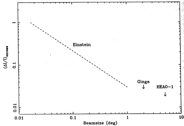
must also contribute to any excess fluctuation signal. We therefore
represent the excess fluctuation results as upper limits
(Figure 5).
,
=
1.5]. Alternatively may be 1.65 in which case
there are no significant excess fluctuations. Clustering (see below)
must also contribute to any excess fluctuation signal. We therefore
represent the excess fluctuation results as upper limits
(Figure 5).
|
Figure 5. Upper limits to excess
fluctuations from P(D) analyses. The
line at ~ arcmin corresponds to the soft XRB and the remaining to
energies |
Correlation analyses of the XRB are also powerful tools for testing source clumping. The autocorrelation function (ACF) of the XRB provides an integrated measure of source extension or clustering on scales greater than the beam. It is defined as
where I is the intensity at one position and
I
The current observational situation is shown in
Figure 6. Only upper
limits were known until recently;
Persic et al (1989)
measured W < 4 x
10-4 on the scale of 3° and Carrera et al
(1991,
1992)
and Martin-Mirones
et al (1991)
found values of W
Figure 6. Upper limits to the
autocorrelation function as a function of
angular separation in degrees. The point at 5 arcmin is tentative and
from ROSAT data
(Hasinger et al 1991;
Chen et al 1991, in preparation)
and refers to 0.1
 is the
intensity at a
position an angle away. An
important feature is that the contribution
of sources to the ACF varies as the square of the fraction they
contribute to the total XRB intensity. The signal in the ACF is
dominated by the brightest sources for angular separations where the
beams overlap - simply reflecting the fact that each individual source
contributes to both beams.
is the
intensity at a
position an angle away. An
important feature is that the contribution
of sources to the ACF varies as the square of the fraction they
contribute to the total XRB intensity. The signal in the ACF is
dominated by the brightest sources for angular separations where the
beams overlap - simply reflecting the fact that each individual source
contributes to both beams.
 10-4 on
scales of ~ 2-3°. Analysis of
Einstein Observatory Imaging Proportional Counter (IPC) data by
Barcons & Fabian (1989)
showed a signal on a scale of about 5 arcmin of W ~ 0.1,
which they treated as an upper limit since the IPC is known to have some
intrinsic irregularities (gain variations in particular) on that scale.
Soltan (1991)
has reduced this limit to 1.2 x 10⁻³, similar to that now
found with ROSAT of ~ 2 x 10⁻³
(Chen & Fabian 1992).
From separations of a
few arcminutes to a few degrees, the best upper limits are provided by
Ginga scans at a level of 1.5 x 10⁻³
(Carrera et al 1992). On larger
scales, a significant detection has been recently reported by
Mushotzky (1992)
who used all the available data from the HEAO-1 A2 all-sky
survey (Figure 2). He finds an ACE
of ~ 3 x 10⁻⁵ on scales from 10-15°
[this is presumably also related to the optical-X-ray cross-correlation
result of Jahoda et
al (1991)
discussed earlier].
10-4 on
scales of ~ 2-3°. Analysis of
Einstein Observatory Imaging Proportional Counter (IPC) data by
Barcons & Fabian (1989)
showed a signal on a scale of about 5 arcmin of W ~ 0.1,
which they treated as an upper limit since the IPC is known to have some
intrinsic irregularities (gain variations in particular) on that scale.
Soltan (1991)
has reduced this limit to 1.2 x 10⁻³, similar to that now
found with ROSAT of ~ 2 x 10⁻³
(Chen & Fabian 1992).
From separations of a
few arcminutes to a few degrees, the best upper limits are provided by
Ginga scans at a level of 1.5 x 10⁻³
(Carrera et al 1992). On larger
scales, a significant detection has been recently reported by
Mushotzky (1992)
who used all the available data from the HEAO-1 A2 all-sky
survey (Figure 2). He finds an ACE
of ~ 3 x 10⁻⁵ on scales from 10-15°
[this is presumably also related to the optical-X-ray cross-correlation
result of Jahoda et
al (1991)
discussed earlier].

E 2 keV. The
continuous line is a 2 upper limit
obtained with the Ginga collimators in scan mode by
Carrera et al (1991b).
Vertical arrows are from Ginga pointed-mode observations
(Carrera et al 1991a);
the detection at 10° is from
Mushotzky (1992) and
the dipole from
Shafer (1983).
 3 keV.