The Full R-Dependent Curve

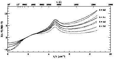
Figure 7 shows the full wavelength range of the IR-through-UV R-dependent extinction curves derived here, for four representative values of R (thick solid and dashed lines). For 2700 Å the curves are computed using the FM fitting function and for > 2700 Å the curves are spline interpolations between the R-dependent spline anchors. The CCM results are shown for comparison by the thin dotted lines for the same four R values. In the UV region, the new results and the CCM curves are similar for R ~4.0, but diverge for larger R. The main reason for this discrepancy lies in the UV linear extinction component. While CCM adopted a linear relationship between the slope c2 and intercept c1, their relation - shown by the dotted line in the bottom panel of Figure 5 - does not agree well with the observations. The large discrepancy at small values of c2 (i.e., large R) produces the difference seen in Figure 7.

Figure 7. Examples of the R-dependent far-IR through UV extinction curves derived in this paper (thick solid and dashed curves). The corresponding values of R are listed on the righthand side of the figure beside the curves. For comparison, the results of CCM for the same four values of R are shown.

A closeup comparison between the new results and CCM in the optical/IR region for the R = 3.1 case can be seen in Figure 6, where the CCM curve is indicated by the dotted line. The disagreement in the region near the Johnson R filter illustrates the bandwidth effect discussed above. The CCM curve is fixed at A() / E (B - V) = 2.32 at 7000 Å, which is taken as _eff for the Johnson R. The new curve is constructed to yield the same value of A() / E (B - V) but for synthetic photometry with the Johnson R. The discrepancy is particularly large for this filter because of the steep change in extinction across its relatively broad profile. This effect also accounts for the lesser discrepancies in the regions of the U, B, I, and J filters. O'Donnell (1994) presented a revision to the CCM formula in the region of the U, B, and V filters based on the Strömgren photometric indices. This revision uses the same stategy as CCM of fixing the extinction ratios at the filter effective wavelengths, but more closely resembles the newly derived monochromatic extinction curve because the bandwidth effects in the narrower Strömgren filters are smaller.

Note that the technique used here to produce R-dependent curves can be used to construct ``customized'' UV/optical extinction curves for sightlines with well-defined UV extinction properties. It is simply necessary to substitute the measured values of A() / E (B - V) at 2700 Å and 2600 Å for the UV spline anchors listed in Table 3 and then perform the cubic spline interpolation to determine the optical portion of the curve, which smoothly joins the measured UV curve at 2700 Å. This method was used in Figure 2 to extend the IUE curves into the optical region.

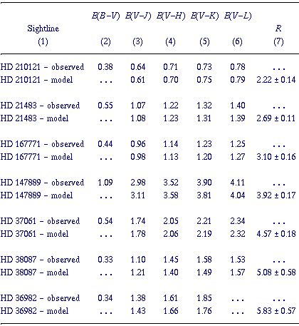
The assertion that the shape of the IR extinction law is invariant can be tested by comparing results obtained from the R-dependent curves in Figure 7 - which were constructed based on this assumption - with observations. This comparison is made in Table 5 for a number of sightlines which span the observed range in R. The ``model'' data listed for each sightline are the results from synthetic photometry on model stellar energy distributions artificially reddened using the R-dependent curves, with E (B - V) values from column 2 of the table and R values from column 7. The listed values of R are those that best reproduce the observed color excesses and the uncertainties result from assuming uncertainties of ±0.02 mag in E (B - V) and ±0.05 mag in the IR E (V-). The agreement between observations and model values is excellent and there are no strong systematic trends evident. The results are thus consistent with an invariant IR extinction curve. At wavelengths greater than ~ 1 µm, the extinction curve roughly resembles a power law with an index of ~ 1.5. This is similar to that adopted by CCM (1.6), but much flatter than that of Martin & Whittet (1990; ~ 1.8).

Table 5. Comparison of Model IR Color Excesses With Observations

NOTE.- Observed color excesses are derived using the intrinsic colors from Wegner 1994. Model color excesses are computed via synthetic photometry of artificially reddened stellar energy distributions using the IR extinction law derived in the Appendix and assuming the E (B - V) values from column 2 and the R values from column 7. The stated values of R yield the best fits to the observed IR color excesses and the uncertainties are based on the assumptions E(B-V) = 0.02 and E(V-) = 0.05. Kurucz ATLAS9 models with appropriate values of Teff were used to represent the intrinsic stellar energy distributions.

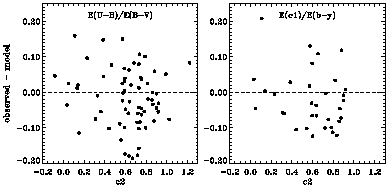
At the blue end of the optical region, the interpolation between the optical and UV spline anchor points can be tested by comparing predictions of the extinction indices E (U - B) / E (B - V) and E (c1) / E (b - y) with photometric measurements. Figure 8 shows this comparison, with the difference between the observed values and predicted values - derived from synthetic photometry of ``customized'' extinction curves from the FM sample - plotted against the slope of the linear component c2. The curves were produced as described above, by adopting the observed values of A() / E (B - V) at 2600 Å and 2700 Å as the UV anchor points. The random scatter (measurement noise) in both indices is large, but no systematic trends are seen and the model curves appear to reproduce at least the integrated properties of extinction well in the near-UV region. Over the range of c2 values shown, the model values of E (U - B) / E (B - V) range from about 0.6 to 0.8 and the values of E (c1) / E (b - y) from about 0.0 to 0.3.

Figure 8. Left Panel: Observed-minus-predicted values of E (U - B) / E (B - V) plotted against the slope of the UV linear extinction component c2 (filled circles) for sightlnes from the FM sample. Model values of E (U - B) / E (B - V) vary over the range ~ 0.6 to ~ 0.8 for the observed range in c2. Right Panel: Observed minus predicted values of the Strömgren extinction ratio E (c1) / E (b - y) plotted against c2 (filled circles) for the FM sightlines with Strömgren data. Model values of E (c1) / E (b - y) vary over the range ~ 0.0 to ~ 0.3 for the observed range in c2.