


5.5. Wide Field Planetary Camera 2 (WFPC2)
WFPC2 (5) was installed on board HST during the first servicing mission in December 1993. Since replacing WF/PC [1] it became the workhorse of the observatory.
WFPC2 is composed of 4 frontally-illuminated CCD cameras. These cameras include optics to correct for the primary's spherical aberration. A pyramidal mirror divides the incident beam and redistributes it among the four fixed cameras. The F/28.3 Planetary Camera (PC) has the highest resolution. The other three, with a F/12.9 and a wider field correspond to the WFC (Wide Field Camera). The WF/PC had eight cameras and the pyramid was able to rotate, selecting the Planetary or the Wide Field cameras.
5.5.1 WFPC2's CCDs
The camera's CCDs have an array of 800 x 800 15µm pixels. Among its characteristics are the ones shown in Table 11.
| Read Noise | 5e- RMS |
| Gain | 7e- /ADU or 14e- /ADU |
| QE at 6000Å (2500Å) | 35% (15%) |
| WFC2, WFC3, WFC4 Resolution | 0.09958, 0.09956, 0.09962"/pixel |
| PC Resolution | 0.04553 "/pixel |
| WFC Field of view | 2.5'x2.5' in an L-shape |
| PC Field of View | 35" x 35" |
WFPC2 is used generally with the 7e- / ADU gain, the most convenient to observe dim objects. If the target is too bright, it is then possible to switch to the higher gain value and then saturating the well with 53000 e- instead of 27000 e-. If the image is saturated, the effects of bleeding or diffraction spikes are observed.
Once a month the camera is heated to eliminate the contaminants that attach themselves to the cool CCDs. In this way the UV sensitivity is regained. This procedure also restores those pixels whose dark counts were abnormally high.
As cosmic rays might be a problem, it is always recommended to split the observations and combine them afterwards, most of them are eliminated in this way. The splitted images can either be at the same position or one slightly displaced from the other. This second method (dithering) has also the additional advantage of restoring the resolution (severely affected by WFPC2's oversampling).
The pipeline corrects most other anomalies seen in the calibration of the raw data.
5.5.2 Filters
The WFPC2 has 48 filters between the 1200Å and 1µm. The list can be found in the camera Handbook. Please see the Instrument Handbook for a complete detail and spectral coverage of the filters.
The camera does not have a continuum of narrow-band filters. Between 3700Å and 9800Å the ramp filters whose wavelength varies with the position are used. Their width is around 1% or 2% of the central wavelength, being useful then to observe objects no larger than 10".
The Quad Filters allow observations in [OII] lines with wavelengths between 3763Å and 3986Å. The Methane Quads and polarizers (with polarization angles at 0°, 45°, 90° and 135°) are harder to use as some positions are lost due to the L-shape of the camera. The camera has also two solar-blind Wood's filters for far UV imaging.
The broad-band filters are similar, but not identical to the Johnson or Cousins ones. Some caution is needed when calculating magnitudes to be sure on what system they are: magnitudes calculated using the header keywords are in STMAG.
5.5.3 What constitutes a WFPC2 observation?
A WFPC2 observation is composed of pairs of files whose name starts with U (WF/PC files start with W) followed by eight alphanumeric characters. The header is a text file whose extension ends with h, and the binary data's extension with d.
These files are extracted from the Hubble Data Archive in FITS format and can be read into GEIS for further reduction and analysis. WFPC2 datasets generally have 4 groups, although sometimes they can have only one if just the image corresponding to the PC was stored.
Tables 12 and 13 summarize the different files corresponding to WFPC2 images. All the files in this table have the same name, only the extension changes.
| extension | class | format |
| d0h/d0d | raw data | integer |
| q0h/q0d | d0h quality files | integer |
| x0h/x0d | engineering data | real |
| q1h/q1d | engineering quality data | integer |
| shh | standard header packet | ASCII |
The only file for which the binary data is not important is the so called standard header packet. Its extension is shh and contains information about the orbit and the different times associated with an observation.
If the data was extracted from the HDA (and not read from a tape) there are two additional files in the dataset with extensions dgr and cgr. These are used to populate StarView tables. They are not used for any data analysis and can be deleted immediately.
The calibration pipeline (or the calwfp task) produces the files shown in Table 13
| extension | class | format |
| c0h/c0d | calibrated data | real (might be integer) |
| c1h/c1d | c0h/c1h data quality | integer |
| c2h/c2d | c0h/c0d histogram | 3 lines (original, A-to-D, calibrated) |
| c3t | photometry table | binary table |
Some header keywords of interest are listed in Table 14:
| RA_TARG, DEC_TARG | Aperture's RA and Dec |
| EXPTIME | exposure time |
| MODE | observing mode (eg., WFALL) |
| ORIENTAT | position angle |
| PHOTFLAM | inverse of the sensitivity |
| PHOTZPT | magnitude zero point |
5.5.4 Calibrated data
As mentioned above, the data stored in the Hubble Data Archive have been processed by the calibration pipeline. If needed, they can be calibrated again using the calwp2 task in STSDAS. Header keywords determine how the calibration will be done.
When the image was constructed in GEIS format (from the original stream received from the spacecraft), these keywords were populated with the names of the best calibration files available at that time. Other keywords were populated with the instructions on how the calibration should be made.
An example of a section of the header of a calibrated file with this information is included below. Only the header of the files is listed, but both the header and the binary data are used for the calibration.
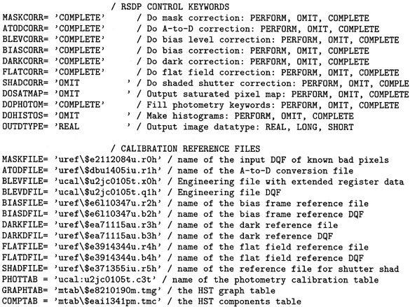
The file with the x0h extension contains, what in ground-based CCD images is the overscan, is known as the extracted engineering data file. For those observations made in FULL mode, it contains 12 columns. The information in this file is used to correct the BIAS level if the parameter BIASCORR = PERFORM. There is a companion file, with extension q1h, whose values indicate the quality of the pixels, as in the case of the science data.
Several files used in
the calibration process are the ones that determine the quality of each
image pixel. Their value comes both from the individual
observation as well as from
the global knowledge of the camera.The file with the q0h
extension indicates each pixel's quality. It is important to recognize
these potentially "bad'" pixels in order to analyze the images correctly.
Table 15 summarizes the values that these pixels
can have in this file, which will help in their identification.
| value | name | comments |
| 0 | goodpixel | "good" pixel will be included in the bias determination and the statistics of the calibrated image |
| 1 | softerror | error generated during the transmission of the data |
| 2 | calibdefect | defect that emerged during the calibration process |
| 4 | staticefect | defect that is common to all WFPC2 images (e.g., dead pixels) |
| 8 | atodsat | problem that emerged during the A-to-D conversion |
| 16 | datalost | the value of the pixel was lost during the data transmission |
| 32 | badpixel | bad pixel that didn't fall in the previous categories |
| 64 | overscan | pixels outside of the region corrected for spherical aberration |
The calibration process generates several files. The most important file is the one with the c0h/c0d extensions, as it is the final result. This file is also paired with quality data files that have c1h/c1d extensions. This last one is the result of the combination (using the logical operator AND of the similar files in the raw and the reference data.
If DOHISTOS = PERFORM a file with extension c2h is created. It contains a histogram of all the good values in the calibrated data. This file contains 3 rows and the same number of groups as the raw file. The first row includes the histogram of the raw data, the second row of the data after the A-to-D conversion and the final one, the histogram of the calibrated data.
The last file created by the calibration process is a table whose extension is c3t. It contains the information needed to populate the photometry parameters in the header (PHOTFLAM, PHOTZPT, PHOTPLAM, PHOTBW). By multiplying the image by the PHOTFLAM value, its units are changed from DN (counts) to flux units. PHOTZPT is the zero point of the system used for the photometry. The other parameters are the wavelength at which the flux was calculated (PHOTPLAM) and the width of the filter (PHOTBW).
5.5.5 The calibration process
The (6) parameters that control the calibration process are part of the image header, as explained above. They can be modified using the STSDAS task stsdas.ctools.chcalpar. If the keyword is set to PERFORM that step of the calibration will be performed. Upon successful completion of this step, the keyword is set to COMPLETE. If the calibration step is skipped, the keyword value is OMIT.
The calibration files appropriate for a given observation can be obtained from StarView's calibration screen (see below).
If MASKCORR = PERFORM the mask flagging defective pixels is included in the c1h file. These bad pixels, bad rows or bad columns, can be studied by displaying this file.
The next calibration step is the analog to digital (A- to-D) conversion, done if ATODCORR = PERFORM. In this case each pixel is replaced by the appropriate value as determined by the corresponding table listed in the header. This table has 3 columns and 8192 rows. One column corresponds to the temperatures in HST's bay 3, the others to the corresponding pixels. For example, the second pixel in the first row is the temperature associated with the second row of the A-to-D table.
If BLVCORR = PERFORM the level of bias is calculated in the x0h file and subtracted from each pixel in the science image. The value for the odd columns is calculated and stored in the BIASODD keyword, while the value for the even ones is stored in BIASEVEN. Each pixel identified as bad is incorporated to the quality file c1h.
The bias image is then subtracted from the science image. This is the calibration file with the r2h extension (and the associated quality file = b2h).
The dark is made as a file with an exposure time of 1 second. This file is multiplied by the header keyword DARKTIME, the value of the accumulation time. This resulting file is subtracted from the science image. The reference file, indicated in the header by the DARKFILE keyword has the r3h extension (the file with b3h extension is the quality file; keyword DARKFIL). If the observation was longer than 30 minutes or more than 4 images were combined so as to obtain a large SNR, it is advisable to use a "superdark". These special files are the combination of 100 individual darks. If a superdark was used, the hot pixels need to be removed using a dark file obtained close to the observation date or creating a mask from the bad pixel lists.
The resulting image from these last operations is multiplied by the flat field (identified in the header by the FLATFILE keyword and with a r4h extension). The flat has already been normalized and its inverse is use to avoid a division by zero.
Finally if SHADCORR = PERFORM the errors caused by the different illumination due to the shutter blades at the entrance pupil. This step is only needed if the observations are shorter than 10 seconds.
As mentioned above if DOPHOTOM = PERFORM the photometry parameters are populated. This is done using the throughput values of the different optical components. These values are calculated using different synphot subroutines.
5.5.6 How to select the "best" reference files
The images obtained with WFPC2 are distributed and archived already calibrated. This calibration was performed with the more adequate reference files available at the time. It is frequent to find out that these are not the "optimal" ones. An example was mentioned above: the "superdarks". The most common one, though, is the existence of new (and probably better) bias and flat fields files. Also, as more details are learned about the instrument, the calibration algorithms are modified. Changes to calwf2 are announced in the Space Telescope Analysis Newsletters and in the WFPC2 WWW pages.
It is always convenient then to be sure that the images are adequately calibrated. The easiest way to check that the appropriate files were used, is to use StarView's calibration screen. As shown in Figure 3, this screen lists the used and suggested files.
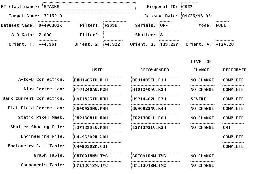
|
Figure 3. The calibration screen for StarView in the HST data reduction process. |
5.5.7 Changing the calibration parameters
As described above, the STSDAS task chcalpar can be used to change the calibration parameters. This task allows to change the name of the files as well as the calibration controls.
The chcalpar parameters are, for example:
   images = "u27L0402T.d0h"  List of images to modify
(template = "")              Image to read header from
(keywords = "")              Pset to use if not reading from an image
     (add = yes)             Add keywords if not present in header?
 (verbose = yes)             Print out files as they are modified?
 (Version = "25Mar94")       Date of Installation
    (mode = "al")
While the pset keywords are:
  maskcorr = "complete")     >do mask correction?
  atodcorr = "complete")     >Do A-to-D correction??
  blevcorr = "complete")     >do bias level correction?
  biascorr = "complete")     >do bias correction?
  darkcorr = "complete")     >do dark correction?
  flatcorr = "complete")     >do flat field correction?
  shadcorr = "omit")         >Do shaded shutter correction?
  dophotom = "complete")     >fill photometry keywords?
  dohistos = "omit")         >Make histograms?
  outdtype = "real")         >output image data type?
  maskfile = "uref\$e2112084u.r0h") >name of the input DQF of known bad pixel
  atodfile = "uref\$dbu1405iu.r1h") >name of the A-to-D conversion
  blevfile = "ucal\$u2jc0101t.x0h") >engineering file with extended register
  blevdfil = "ucal\$u2jc0101t.q1h") >engineering file DQF
  biasfile = "uref\$e6l10347u.r2h") >name of the bias frame reference file
  biasdfil = "uref\$e6l10347u.b2h") >name of the bias frame reference DQF
  darkfile = "uref\$ea71115au.r3h") >name of the dark reference file
  darkdfil = "uref\$ea71115au.b3h") >name of the dark reference DQF
  flatfile = "uref\$e3914344u.r4h") >name of the flat field reference file
  flatdfil = "uref\$e3914344u.b4h") >name of the flat field reference DQF
  shadfile = "uref\$e371355iu.r5h") >name of the reference file for shaded sh
   phottab = "ucal:u2jc0101t.c3t")  >name of the photometry calibration table
  graphtab = "mtab\$e8210190m.tmg") >the HST graph table
   comptab = "mtab\$eai1341pm.tmc") >the HST components table
instrument = "wfpc2")      Instrument represented by this pset
   Version = "14Feb94")    Date of Installation
      mode = "al")
The control parameters can be changed to PERFORM (to execute), OMIT, if that part of the calibration will be omitted. The recommended flat field needs to be extracted from the HDA before proceeding with the calibration, and its name entered in the pset.
5.5.8 Continuing the reduction
The reduction process can continue after the calibration. Several steps can be taken depending on the desired final results.
5.5.9. Cosmic Rays
Probably the next step is the elimination of the cosmic rays. This is not an easy task as, due to the undersampling, point sources can be confused with a cosmic ray.
To eliminate the cosmic rays in an image, the stsdas.hst_calib.wfpc2.crrej task can be used to combine a pair of CR-SPLIT images. An example of the parameters of this task is:
infile = "u*.c0h"      >input images
  outfile = "3c353"    >output image name
 outfile2 = ""         >output (number of good points) image name (opt
   sigmas = "5,5,4,3"  >rejections levels in each iteration
   radius = 0.         >CR expansion radius in pixels
  pfactor = 0.         >CR expansion discriminator reduction factor
hotthresh = 4096.      >hot pixel threshold in DN
   minval = -99.       >minimum allowed DN value
  initial = "min"      >initial value estimate scheme (min, med, or fi
 noisepar = "")        >Noise model parameters (pset)
  fillval = INDEF)     >fill value for pixels having CR in all input i
 (verbose = yes)       >print out verbose messages?
     mode = "al")
The pset in this case is:
(readnoise = 0.85)     Read noise (in DN) from noise model
      gain = 7.)       Detector gain in electrons/DN
scalenoise = 5.)       Multiplicative term (in percent) from noise mod
      mode = "al")
5.5.10. Orientation
The position angle is stored in the ORIENTAT header keyword. Although the image can be easily rotated so as the North direction is up (and East is left), it is easier to start the analysis using the stsdas.graphics.sdisplay.compass task. It draws an arrow pointing North.
To combine the four images (each in one group) and obtain an image with the full WFPC2 field of view, it is possible to use the stsdas.hst_calib.wfpc2.wmosaic task. The resulting image has not been rotated to have North at the top.
5.5.11. Positions
Images obtained with the WFPC2 suffer from a geometric distortion due to the optics and the physical characteristics of the camera. This distortion varies with the position of the pixel, being smaller close to the center of the chip and around 3-4% at the edges. To measure absolute positions in a WFPC2 image, it is necessary to account for this effect. The task stsdas.hst_calib.wfpc2.metric is the recommended one to perform position measurements. The task rimcursor can be used to measure positions in images resulting from wmosaic. The precision of the relative measurements is between 4 and 10 milli-arcseconds. The absolute measurements are as "good"as the ones from the guide stars used to point the telescope while obtaining the image. The nominal error of the Guide Star Catalog (GSC) is 0.7".
In the case of the so-called early acquisition images it is necessary first to locate a common star in the WFPC2 and GSC plate images. The offset, if existent between these two positions can be determined and then applied to the absolute measurement of the target. This position is then the one used to point the spectrograph.
5.5.12. Photometry
To convert the DNs into magnitudes, in principle, only the following formula can be used:
where
PHOTOZPT
is the magnitude zero point. Its value (and the corresponding PHOTFLAM)
are included in the header. This system is based in a spectrum with a constant
flux per wavelength. In this case the flux density is simply:
The values obtained in this
way, need to be corrected still for temporal and spatial defects, as for
example those due to:
A detailed description can be found in
Holtzman et al. (1995).
For more details and examples please
see the WFPC2 photometry page at
http://www.stsci.edu/instruments/wfpc2/Wfpc2_phot/wfpc2_cookbook.html
With the task synphot the different magnitude values can be estimated.
Without much additional
work, it is possible to obtain magnitudes with a 5% error. By using more
precise models and performing all the necessary corrections the errors
are reduced to 2% or 3%.
5.5.13. Conversion from STMAG to Johnson's UBVRI and Cousins' RI
The following table can
be used to convert the magnitudes obtained with the formula above to the
Johnson's or Cousins' systems. The values listed in the table were obtained
using synphot and
have errors ~ 5% (probably larger in the U band). Different
Bruzual models were used (see the synphot
manual) to create this table as the correction depends on the class of
the object. For more details see the Photometry documents in the WFPC2
WWW pages.
The following tasks can be
used to plot the different filter throughputs and compare them:
To generate one of the entries of the table, the command is
Where band(wfpc2,1,a2d7,f336w) defines the F336W band;
band(johnson,u) is Johnson's U band and crgriddbz77$bz_1
is an O5 V spectrum from Bruzual's model
library. The entries in the table are the
differences between these
two values. The errors are ± 0.05mag (probably larger in the UV).
Example
The magnitude of an M6
V star observed with the WF4 needs to be calculated in Cousins I band.
From the header parameters
Then,
From the previous table, the
correction value for this case is -1.21, then
The measured counts can then
be converted to magnitudes in the Cousins band using
If the star had 115 counts/sec, then the magnitude is I = 16.50mag.
Note that all these calculations
were performed with the counts measured as count rates. Some photometry
programs expect counts in units of exposure time. In this case, then the
magnitude zero point is
5 Please refer to the WFPC2 Intrument
Handbook for complete details of the instrument. It can be found at
http://www.stsci.edu/instruments/wfpc2/wfpc2_top.html
Back.
6
Please refer to the HST Intrument Handbook for a complete description of
the calibration process for HST data. Back.
U-F336W
B-F439W
V-F555W
R-F675W
I-F814W
R-F675W
I-F814W
O5 V
0.53
0.67
0.05
0.67
1.11
0.71
1.22
B0 V
0.46
0.66
0.05
0.67
1.13
0.70
1.22
A0 V
0.08
0.67
0.02
0.68
1.22
0.67
1.21
F2 V
0.03
0.62
0.00
0.69
1.28
0.63
1.22
G0 V
0.02
0.58
0.01
0.70
1.31
0.60
1.23
K0 V
0.10
0.53
0.01
0.69
1.32
0.58
1.23
M0 V
0.04
0.43
0.00
0.78
1.48
0.54
1.22
M6 V
0.05
0.29
0.03
1.05
1.67
0.56
1.21
sy> plband "band(wfpc2,1,a2d7,f814w) left=6000 right=12000 norm=yes
ltype=solid dev=stdgraph


sy> plband "band(johnson,i)" normali+ ltype=dashed append+
device=stdgraph


sy> plband "band(cousins,i)" normali+ ltype=dashed append+
device=stdgraph
sy> calcphot "band(johnson,u) crgriddbz77\$bz\_1 vegamag
sy> calcphot "band(wfpc2,1,a2d7, f336w)" crgriddbz77\$bz\_1 stmag