5. STATISTICS OF LARGE-SCALE STRUCTURE

In the previous sections we have mostly limited our discussion to the observed general characters of the large-scale structure of the Universe within z < 0.2, as described by the distribution of luminous objects. The visual appearance of large-scale structures - while very interesting per se - needs to be translated into a quantitative description through the application of statistical estimators of clustering if one wants to compare the data to model predictions.

The increased size of galaxy and cluster redshift samples that we have discussed in the previous sections, has in parallel given the possibility to produce more and more accurate estimates of the two-point correlation function and the power spectrum of the distribution of these objects. This has allowed us to start looking at the details of the shape of these functions, in particular on large scales, where we have seen they are more interesting for the theory. Such details, if confirmed, can have profound consequences for our understanding of the origin of large-scale structure, as I shall try to summarize and discuss in this section.

5.1. The Galaxy Two-Point Correlation Function

The simplest approach to clustering is to ask how much does it differ from a uniform distribution at the two-point level, or in other words, which is the excess probability over random to find a galaxy at a separation r from another galaxy. This is one way in which the two-point correlation function (r) can be defined (see [72] for a more detailed introduction). The first estimates of the two-point correlation function go back to the seventies [73], but the lack of large redshift samples limited these early analyses to the angular correlation function w(). This is related to (r) through the Limber equation [72]

(2)

where is the radial selection function expected for the 2D survey being analysed.

The basic description of galaxy clustering that emerged from these works is still valid today on small and intermediate scales: w() is well described by a power law ^-0.8, corresponding to a spatial correlation function (r / r₀)^-, with r 5 h^-1 Mpc and - 1.8, and a break with a rapid decline to zero around r ~ 10 - 20 h^-1 Mpc. As we shall discuss in the following, modern surveys have significantly improved our knowledge of the two-point correlation functions especially on scales > 10 h^-1 Mpc. However, before discussing these most recent results, it is important to briefly describe how galaxy peculiar velocities affect the observed shape of (r) .

5.1.1. REDSHIFT SPACE DISTORTIONS   The actual detection of true intrinsic deviations of (s) from a power law is complicated in the analysis of redshift surveys by the effects induced by galaxy peculiar velocities. Here s is now used to make it explicit that separations are in reality not measured in true 3D space, but in redshift space: what we actually measure when we take the redshift of a galaxy is the quantity cz = cz_true + v_pec//, where v_pec// is the component of the galaxy peculiar velocity along the line of sight. This component, while typically ~ 100 km s^-1 for ``field'' galaxies, can rise above 1000 km s<sup>-1</sup> in rich clusters of galaxies. This distorts the real-space correlation function in different ways, depending on the scale. The resulting (s) , is in general flatter than the real-space (r) . This is the result of two competing effects: the small-scale pairwise velocity dispersion, mostly dominated by high-velocity pairs in clusters of galaxies (i.e. those within the so-called ``Fingers of God''), damps the amplitude of (r) below ~ 3 h^-1 Mpc. On the other hand, coherent flows towards large-scale structures enhance the contrast of those structures lying perpendicularly to the line of sight, thus amplifying (s) in the linear regime (i.e. above 10 - 20 h^-1 Mpc). I will not enter here into details on how the wealth of information on the dynamics of galaxies contained in these distortions can be extracted, but limit myself to a discussion on how to correct them to recover the true shape of (r) . A more complete discussion can be found, e.g., in [74] and [51].

Redshift space distortions can be corrected either at a rough level, through a simple statistical compression of the ``Fingers of God'' (e.g. [75]), or in a more appropriate way by computing the correlation function (r_p, ) , where the separation vector s between two objects is split into two components r_p and related as s² = r_p² + ². This two-dimensional correlation function can then be projected along the line-of-sight direction, to obtain the function

(3)

which is independent of redshift-space distortions. We have already encountered this function in Figure 6 when comparing the clustering strength of early- and late-type galaxies in real space (and thus free of their rather different peculiar velocity fields). w_p(r_p) can either be used to constrain the parameters of a chosen model for (r) , as e.g. the classical (r) = (r / r₀)^- [56], or inverted through the Abel integral relations to recover the whole (r) .

All these problems are obviously absent when one analyses w(), where on the other hand the strongest uncertainty in the de-projection lies in the knowledge of the radial selection function.

5.1.2. THE LARGE-SCALE SHAPE OF (r)   The simple form observed from the first estimates of w() and (r) at small separations was consistent with the expectations of gravitational growth from some initial spectrum of fluctuations (at the time thought to possibly be a simple white-noise i.e. k⁰, see next section): as gravity has no built-in preferential scale, a power law seemed to be a natural consequence of gravitational clustering (see e.g. [72]). However, since then we have understood that plausible initial conditions are all but a white-noise (see e.g. the first computation of the linear power spectrum in a Universe dominated by Cold Dark Matter, [76]), so that the clustering we measure today with (r) is not just the product of the nonlinear action of gravity.

In Figure 9, I have plotted the estimates of (s) for the ESP [77, 32], the LCRS [78], the Stromlo-APM (Loveday et al. 1992b), and the Durham-UKST [80] surveys. These samples represent a selection of data that should offer the best compromise between depth and angular aperture, thus maximising the ability to sample large scales. In addition, the dotted lines show a plot of (r) obtained through de-projection of the angular w() from the APM galaxy catalogue [81] under two different assumptions about galaxy clustering evolution and thus selection function.

Figure 9. Recent estimates of the two-point correlation function of optically-selected galaxies. The plot shows results from the ESP (Guzzo et al. 1998, 1999), the LCRS (Tucker et al. 1997), the APM-Stromlo [79] and the Durham-UKST [80] surveys.

The global form below 5 - 10 h^-1 Mpc is still well described by a power law: the slope is very close to the classical -1.8 for the APM (r) , which is in real space, while it is flatter for all the redshift-space measures due to the suppression by peculiar velocities discussed above. Above ~ 5 h^-1 Mpc there is unanimous evidence for more power than expected by a simple extrapolation of the small-scale slope. This ``bump'' or ``shoulder'' is evident both in the APM (r) and in the redshift-space measures, implying that it is not an effect of the expected redshift-space amplification by coherent flows [82]. We found clear early evidence for this excess when studying clustering in the Perseus-Pisces survey [47], and realised that it was present already in the published CfA1 data (as also noticed in [83]). At the time we suggested that it was and indication for a steep power spectrum P(k) k^-2.2 on large scales. Further theoretical modeling [84] and the new direct measures of P(k) in real space from the APM survey [85], confirmed that indeed there is a significant change in (r) around r 3 - 5 h^-1 Mpc. It was natural to interpret this as a consequence of the transition between the strongly nonlinear clustering regime at small separations, to a quasi-linear regime on larger scales. In Section 5.3 we shall come back to this point while discussing directly the observed shape of P(k).

5.2. The Clustering of Clusters

We have seen that clusters of galaxies represent a powerful tracer of structure on the largest possible scales. Their clustering can be also quantified at the simplest level through the two-point correlation function. The classic estimate of (s) for Abell clusters [86] showed that the cluster-cluster correlation function is also well described by a power law, with a slope apparently similar to that of galaxies, but a correlation length about 4 times larger. In reality, due to the limited size of the sample, the original fit was performed imposing a slope = 1.8, and therefore it was not really a measure of the functional shape of cluster-cluster correlations. Nevertheless, the fit was good enough, and it became generally accepted that the cluster-cluster correlation function has a the same slope as galaxies, = 1.8, but larger amplitude (see e.g. [60]), that is _cc(r) A . _gg(r). In fact, this statement could not rigorously be true if a simple statistical amplification mechanism, as then suggested by Kaiser [60], were the origin of the different amplitude: clusters trace scales > 10 h^-1 Mpc, i.e. cover mostly fluctuations that are in the quasi-linear or linear regime, and it would have been a rather strange conspiracy, that their slope were the same that galaxies display on scales between 0.1 and 5 h^-1 Mpc, where clustering is highly nonlinear.

The basic problem was that the galaxy correlation function was not known accurately enough on large scales, as to provide a meaningful comparison. The situation has fortunately improved significantly since then. We have just reviewed the significant progress made in our knowledge of the galaxy correlation function. In parallel, new cluster samples have been constructed, such as the EDCC [87] and APM [89] automatically selected cluster catalogues, and the quality and number of redshifts available for Abell clusters have substantially increased.

Although I will not enter into details concerning optically-selected clusters, in Figure 10 I have reproduced a plot from [61], showing an up-to-date comparison of the cluster-cluster correlation functions of both an Abell sample [88], and a sample of APM clusters [89]. While comparison is presented with two possible power laws, the data clearly show a break from these simple models around 50 h^-1 Mpc, much in the same way as galaxies do on a similar scale. See [61] for more details.

Figure 10. The cluster-cluster correlation function optically-selected clusters from the Abell and APM catalogues, reproduced from the review by Postman [61].

In section Section 4.1 I argued that X-ray selection is the best way to select homogeneous samples of clusters with well-defined physical criteria out to large redshifts. In particular, X-ray luminosity is a parameter that is much more closely related to mass than the somewhat loosely defined richness, used to characterise optically-selected clusters. For this reason, model predictions for the clustering of massive objects, can be more easily and safely translated in terms of observable quantities as luminosities and fluxes, than in the case of galaxies [90]. At a simpler observational level, it is particularly interesting to compare _cc for X-ray selected clusters to that of galaxies, as we do in Figure 11 [91]. This figure shows a preliminary estimate of _cc from the flux-limited REFLEX survey [92], compared to the galaxy-galaxy correlation function from two volume-limited subsamples of the ESP survey [32] ⁽¹¹⁾ . The dashed line on top of the cluster points is the Fourier transform of the power spectrum of REFLEX clusters (computed independently, see next section) while the bottom line has been scaled down by an arbitrary factor b_cg² = (3.3)², so as to overlap the galaxy points. The agreement between the shapes of the cluster and galaxy correlation functions is remarkable. Here we also see how a proper functional description of the shape is not just a simple power law. The one shown here is the Fourier transform of the simple phenomenological shape for P(k) suggested by Peacock [51].

The result shown in Figure 11 is a powerful confirmation of a simple linear bias model between galaxies and clusters of galaxies, analogous to eq. (1), as first suggested by Kaiser [60] (see also [93] for a more recent refinement). Indeed, considering the relationship between (r) and the variance within a top-hat sphere of radius r

(4)

eq. (1) implies that the cluster and galaxy correlation functions obey to the relation

(5)

where the relative bias factor b_cg is related to the typical mass of the clusters considered [60]. This kind of investigation can be generalised to the study of the dependence of the correlation length on the sample limiting X-ray luminosity, for which also model predictions can be quite specific [93]. This will also be an important output of the REFLEX survey [92].

Figure 11. Comparison of the two-point correlation functions of REFLEX clusters [92] and ESP galaxies [32]. The top dashed line is the Fourier transform of a simple phenomenological fit of the REFLEX power spectrum with a double-power-law model. The bottom one is the same after scaling by an arbitrary bias factor of bc2 = (3.3)2. The agreement in shape between galaxies and clusters is remarkable. At the same time, both galaxies and clusters show an indication, after the breakdown around r 50 h-1 Mpc, for more positive power on scales exceeding 100 h-1 Mpc.

5.3. The Power Spectrum

The Fourier transform of the correlation function is the power spectrum P(k)

(6)

which describes the distribution of power among different wavevectors or modes k = 2 / once we decompose the fluctuation field = / over the Fourier basis [51].

The amount of information contained in P(k) is thus formally the same yielded by the correlation function. The estimates of P(k) or (r) from redshift surveys, however, are affected in different ways by uncertainties introduced, for example, by the poor knowledge of the mean density (in which case the power spectrum is to be preferred), or by the shape of the survey volume (whose effect is usually more easily treated when computing (r) rather than P(k)). Useful references for learning more about this topic are [94], [7] and [51], where further directions can be found to specific technical papers. One practical benefit of the description of clustering in Fourier space through P(k) is that for fluctuations of very long spatial wavelength ( > 100 h^-1 Mpc), where (r) is dangerously close to zero and errors easily make the measured values fluctuate around it, P(k) is on the contrary very large. Around these scales, most models predict the power spectrum to have a maximum, which reflects the size of the horizon at the epoch of matter-radiation equivalence.

Indeed, comparison of observations to the theory is in principle easier and more direct using P(k). First, models are usually specified in terms of a linear P(k), which is the result of the action of the specific transfer function of the model on a primordial spectrum, usually assumed to be of the so-called Harrison-Zel'dovic scale-invariant form k¹, which is also the kind of spectrum most naturally produced in inflationary scenarios (see e.g. [50] for more details). In addition, k-modes in Fourier space are statistically independent (a part from the convolution effects due to the window function of the survey, see below), and direct ² comparisons to models is feasible, which is in principle not the case when the correlation function is analysed (see e.g. [95]).

However, not everything is better with power spectra. Redshift surveys are all but cubes (i.e. what would be optimal for a Fourier plane-wave decomposition), and their geometrical shape affects the measured power, so that what we really measure is the quantity

(7)

The measured power spectrum is therefore a convolution of the true P(k) with the square modulus of the window function |W(k)|² , that is the Fourier transform of the survey volume, plus an additional shot-noise term. While the shot-noise contribution SN is easily corrected for, the recovery of the true P(k) necessarily involves a delicate de-convolution operation in k space. While for nearly tridimensional surveys (as IRAS-based surveys [96, 97, 98], or the CfA2-SSRS2 [99], Stromlo-APM [100], Durham-UKST [101], and REFLEX surveys), the effect of the window function is mostly negligible, for nearly two-dimensional surveys as the LCRS or, even worse, the ESP, its effect is dramatic to very small wavelengths. The key point is that for slice surveys like ESP, the window function is very anisotropic, in particular it is extremely large along the direction perpendicular to the main plane of the survey. When the final estimate of P(k) is computed by averaging over the whole 4 solid angle, this anisotropy brings contributions from different k's into the same averaged k bin. It is important to keep these limitations in mind when one compares estimates of P(k) from different surveys as we shall do here. A comprehensive discussion on different estimators for P(k) and how to take these effects into account can be found in [102].

A different approach for dealing with surveys with peculiar shapes is otherwise that suggested by Vogeley & Szalay [103], using the so-called Karhunen-Loève transform. Rather than trying to correct the effect of the window function over the plane waves of the Fourier basis, the idea is to find a different set of orthonormal eigenvectors which are optimal given the survey geometry. The interesting quantities, as e.g. P(k), are then projected on this basis, both for the data and for the models, and comparison is performed through a maximum likelihood analysis. Application of this method has been so far limited only to the 2D case [103]. A first application to the REFLEX data [105] is yielding promising results.

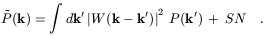
5.3.1. THE POWER SPECTRUM OF THE GALAXY DISTRIBUTION   In Figure 12, I have plotted the estimates of P(k) for the same surveys as given in Figure 9 ⁽¹²⁾ . The four data sets allow me also to make a comparison of estimates from relatively tridimensional surveys (Stromlo-APM, Durham-UKST), to more bidimensional samples as the LCRS and ESP, the latter being in practice a single thin slice cut through the galaxy distribution. This means that the effect of the window function (and the need of a proper correction) on these data sets is very different. In addition, three of the four samples are selected in exactly the same photometric band, the blue-green b_J (two, ESP and Durham-UKST are even constructed from the same catalogue, the EDSGC), the only exception being the r-band selected LCRS. This has the positive effect of reducing the relative biasing between the different samples, although some effect is possibly still present due to the different luminosity ranges covered.

Figure 12. A non-exhaustive compilation of most recent estimates of the power spectrum of galaxy clustering, from four of the largest available redshift surveys of optically-selected galaxies (ESP [106]; LCRS [107]; Stromlo-APM [100]; Durham-UKST [101]), compared to that deprojected (and therefore in real space), from the 2D APM galaxy survey [85].

In the same figure, I have also plotted (dashed line) P(k) as reconstructed from the projected angular clustering of the APM galaxy catalogue [85]. This is clearly the only estimate which is free of redshift-space distortions. The effect of these is shown in particular by the slope above ~ 0.3 h Mpc^-1: an increased slope in real space (dashed line) corresponds to a stronger damping by peculiar velocities, diluting the apparent clustering observed in redshift space (all points).

The first impression from this comparison is that to first order there is quite a good agreement across the different samples. The general trend is that of a well-defined power law range between ~ 0.08 and ~ 0.3 h Mpc^-1, with a slope around k^-2. Note that despite these samples are rather similar in terms of their galaxy properties, a minimal level of relative biasing might be present because of the relative weight of faint and bright objects. The only two samples that should in principle display the same amplitude are the ESP and the Durham-UKST surveys, which are both selected from the EDSGC catalogue. In fact, their P(k) are practically identical over a good range of k's. On one hand, the Durham-UKST P(k) becomes rather noisy at small scales, due to the sparse sampling strategy of this survey (less sparse than the Stromlo-APM, though). On the other hand, the ESP P(k) performs well on small scales, but on large scales it has to be limited to k > 0.06 h Mpc^-1, below which the effect of its nasty window function cannot be deconvolved appropriately. In fact, the very good agreement with the Durham-UKST down to fairly small k's is a very encouraging indication of the quality of the deconvolution procedure performed by the authors [106].

We also note how the LCRS power spectrum tends to be flatter and of lower amplitude around the tentative turnover displayed by the Durham-UKST and Stromlo-APM spectra. Also at large k's, where ESP and Durham-UKST are significantly damped by small-scale pairwise velocities, the LCRS P(k) seems to be less affected by this distortion. The same trend is also visible in the correlation function plot of Figure 9.

Recalling the discussion of Section 5.1 on the shoulder observed in the two-point correlation function above ~ 5 h^-1 Mpc, here we can see clearly the same effect in P(k) by looking at the real-space power spectrum from the APM catalogue. The slope of the APM P(k) above 0.3 h Mpc^-1 is ~ k^-1.2, corresponding to the small-scale clustering regime (in real space!) where - 1.8. Below this scale, P(k) steepens to ~ k^-2, and this is what produces the excess power in (s) on large scales.

Peacock [108] applied the sophisticated linear reconstruction machinery by Hamilton and collaborators [109] to the whole P(k) from the APM catalogue (and to another real-space estimate from the the IRAS-QDOT survey [110]) and concluded that the shape was indeed consistent with a linear power spectrum characterised by a steep slope (~ k^-2.2). This is the same value of linear slope originally suggested in [47] to explain the observed large-scales shape of (s) in the CfA1 and Perseus-Pisces redshift surveys, and confirms the early speculation that the observed change in slope of (r) is a manifestation of the transition from the quasi-linear to the strongly nonlinear clustering regime.

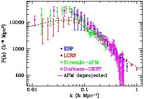
5.3.2. THE POWER SPECTRUM FROM CLUSTERS   Also for measuring the power spectrum, clusters of galaxies offer the most efficient alternative to galaxies, given their ability to sample very large volumes. A first preliminary estimate of P(k) from the REFLEX survey is shown in Figure 13 [105], compared to the power spectra of the largest redshift sample available for Abell clusters [111], and that of the APM automatic optically-selected clusters [112]. This is a conservative measure, based on only 188 of the nearly 460 clusters with redshifts that will form the final REFLEX sample, using a Fourier box of 400 h^-1 Mpc comoving side. This was done to avoid possible spurious fluctuations due to the incomplete sampling between the Northern and the Southern galactic sides of the survey. At the time of writing this review, virtually all clusters in the survey have been observed spectroscopically. A new measure of P(k) in a box of ~ 1000 h^-1 Mpc side (i.e. using all clusters within z ~ 0.2, where the survey is complete), should be produced by the end of 1999 ⁽¹³⁾ . Despite the point at smaller k's is not significant, the turnover around k 0.05 h Mpc^-1 is shown to be significant at the 3 level by a Karhunen-Loéve [103] Maximum Likelihood analysis ⁽¹⁴⁾ . The analysis of the whole survey should also allow to put more serious constraints on the detailed shape of P(k) around the turnover.

Figure 13. The power spectrum of the clustering of clusters, as measured from three different cluster surveys: a preliminary subsample of 188 clusters from the X-ray selected REFLEX survey [105], and redshift samples from the Abell [111], and APM [112] cluster catalogues. Note that a systematic difference in amplitude among these surveys is expected as they sample different mass thresholds, and are therefore characterised by different bias values.

5.4. Features in the Power Spectrum

During the last few years, evidence has indeed been accumulating that the peak of the power spectrum could be rather sharp, perhaps characterised by an extra feature (with respect to smooth traditional models) around its maximum. Einasto and collaborators [114] analysed the distribution of Abell clusters, finding evidence for a sharp peak around k 0.05 h Mpc^-1. Although their result was questioned by other workers because of the possible incompleteness in the sample and the way P(k) was estimated, the presence of such a feature was confirmed by a more conservative reanalysis of Abell data [111], where a slightly less pronounced but still significant peak is found, as we show in Figure 13. The peak is indeed evident in the Abell data, while the preliminary REFLEX sample is not yet able to put serious constraints on the shape around the turnover. Note also the very good agreement of the slopes of the three power spectra above k 0.5 h Mpc^-1, and at the same time the shift in amplitude of the three samples. The latter is a clear manifestation, again, of the different bias of the three samples. An X-ray selected sample as REFLEX allows for a more direct link to the typical mass of the objects we are looking at (see [115], for a more extended discussion of these points).

If we also recall that evidence for excess power around ~ 100 h^-1 Mpc was provided by a 2D power spectrum analysis of the LCRS slices [116], we cannot avoid being amused by the consistency in the peak scale to which these separate measures point, i.e., consistently between 100 and 150 h^-1 Mpc. This is remarkably close to the ``periodicity'' scale revealed by Broadhurst and collaborators ([117], BEKS hereafter), in the analysis of their 1-dimensional pencil-beam surveys towards the galactic poles. This latter result has certainly been one of the most exciting findings of this decade in the study of large-scale structure. The authors merged together two deep redshift surveys of redshifts performed independently in the direction the two galactic poles over a small field of ~ 0.7 degrees, exploring a total 1-dimensional baseline of ~ 2000 h<sup>-1</sup> Mpc. The resulting galaxy distribution showed a surprising regularity of ``spikes''. The visual impression was quantified and confirmed by a 1D correlation and power spectrum analysis, that clearly indicated a preferential ``fluctuation'' at 128 h^-1 Mpc.

This result originated significant controversy. It was suggested that it could just be an aliasing of power due to the small size of the beam, that projected power from small to large scales [118]. On the other hand, the reality of the effect was supported by independent observations showing how the more nearby peaks detected in the pencil beam were coincident with known, real large-scale structures, as the Great Wall or the Sculptor supercluster (e.g. [119]). Further pencil beams in different directions (e.g. [120]), and a denser sampling around the original pointings [121] also show that, yes, this direction is somewhat special, but only in the sense that here the effect is maximised. This is what one would statistically expect if there is indeed a distribution of typical ``cell'' sizes around a characteristic dimension [122]. The peak observed in the 3D power spectrum of Abell clusters around the same scale is further suggesting that the origin of the BEKS periodicity lies indeed in a specific feature in the 3D power distribution around this wavelength.

Note also in Figures 9, 10 and 11 the behaviour of the two-point correlation functions on very large scales, for both galaxies and clusters. Although the binning of (s) is very coarse at these separations, there is a hint that (s) becomes positive again around 150 - 200 h^-1 Mpc. This seems to be common to nearly all surveys, independently of their geometry (slice or 3D surveys), the kind of tracer (galaxy or clusters), and the estimator used. As can be readily seen by Fourier transforming a ``standard'' P(k) (e.g., a CDM shape [123]), this damped oscillation of (s) cannot be reproduced if P(k) has a smooth turnover around its maximum, and seems to be a further hint for a sharp peak. A similar oscillation in the correlation function was claimed for Abell clusters [124], and interpreted as evidence for a sharp feature in P(k).

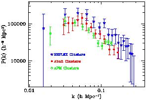
At the time of writing this review (Spring '99), one very interesting piece of evidence has been provided along the same lines by Broadhurst and Jaffe [125], who analyse the redshift distribution of the high-redshift samples of Lyman-break selected galaxies by Steidel and collaborators [57]. As shown in Figure 14, they find again the same effect detected at smaller redshift, i.e. the emergence of a preferred clustering scale. One important consequence is that the co-moving scale of the peak in the power spectrum measured locally ( ~ 130 h^-1 Mpc), can be used as a standard stick to provide a constrain on the combination of _M and : 48_M - 15 10.5, which for a flat Universe (_M + = 1), gives _M = 0.4 ± 0.1.

Figure 14. The one-dimensional clustering of Lyman-break galaxies, from [125]. Left: the co-added pair counts from 5 fields at z ~ 3 (top histogram), compared to the expectations from a randomly distributed sample with the same selection function (solid line). Right: the 1D correlation function along the line of sight, showing the clear pattern with ~ 130 h-1 Mpc periodicity (using = 0.2). See [125] for details.

The convergence of so many independent observations seems to have left little doubt, in my opinion, that the observed characteristic scale is real, and is telling us something important about the properties of our Universe. Indeed, on the theory side there has been considerable interest in the recent literature about the possibile relation of this peak to baryonic acoustic features produced within the last scattering surface at z ~ 1000, when the Cosmic Microwave Background (CMB) radiation originated. Eisenstein and collaborators [126], show however how a large baryon fraction (_b / ₀ 0.3 or larger), and a rather ad hoc combination of parameters (as e.g. a ``blue'' tilt of the primordial spectrum) are required to match the observed Abell peak, while at the same time being consistent with the cluster abundance <sup>(15)</sup> . More dramatically, it is worrying to see that no realistic CDM parameter combination is capable to account for the excess power (the ``shoulder'') we were discussing in section 5.1, that is displayed by virtually all modern surveys [127].

Even without considering the existence of extreme features, therefore there seems to be a general difficulty for the ``standard'' theory to explain the detailed shape of P(k), now that the data are becoming of higher and higher quality in the linear regime. Especially when one tries matching the power spectrum implied by the growing amount of CMB anisotropy experiments to that displayed by the clustering of luminous matter, problems seem to be unavoidable. According, for example, to Silk & Gawiser [128] ``If the data are accepted as being mostly free of systematics and ad hoc additions to the primordial power spectrum are avoided, there is no acceptable model for large-scale structure.'' Once again, a major uncertainty prevents any firm statement from being made: are we allowed to compare the power spectrum derived from the distribution of light to that derved from the mass (CMB), through a simple linear bias scaling? Clearly, a scale-dependent bias would add room for any detailed match between models and the data, but without a solid physical basis would also add an unpleasant ad hoc taste to the whole picture. In addition, the extremely linear relation between the correlation functions of galaxies and clusters that we have shown in Figure 11, seems to suggest that at least above ~ 5 h^-1 Mpc the galaxy and mass distributions are linked by a simple linear bias.

¹¹ The use of volume-limited samples is to be preferred when discussing the shape of (s) . Estimates of (s) from whole magnitude-limited surveys are normally subject to weighting schemes, as e.g. the so-called J3 minimum-variance weighting, which, while allowing a better sampling of very large scales, can affect the globale shape of (s) (Guzzo et al. 1999). Volume-limited samples are much better defined in terms of the properties of the galaxies they include, containing only objects with luminosity above a well-defined threshold. Back.

¹² One further notable estimate, not shown here, has been recently produced from the IRAS-based PSCz survey, and can be found in [104]. Back.

¹³ Note added in proof: a new estimate of P(k) within such a volu me obtained just before completing the final version of this paper, can be found in [113] Back.

¹⁴ That is, projecting the data and a phenomenological form for P(k), with two power laws connected at a scale x_c, over the best basis of eigenvectors found for the REFLEX geometry [105]. Back.

¹⁵ Note added in proof: a similar model is found to provide a good description of the most recent estimate of P(k) from the REFLEX data [113]. Back.