


6.1. Production during inflation
The ability of inflation to generate perturbations on large scales comes from the unusual behaviour of the Hubble length during inflation, namely that (by definition) the comoving Hubble length decreases. When we talk about large-scale structure, we are primarily interested in comoving scales, as to a first approximation everything is dragged along with the expansion. The qualitative behaviour of irregularities is governed by their scale in comparison to the characteristic scale of the Universe, the Hubble length.
In the big bang Universe the comoving Hubble length is always increasing, and so all scales are initially much larger than it, and hence unable to be affected by causal physics. Once they become smaller than the Hubble length, they remain so for all time. In the standard scenarios, COBE sees perturbations on large scales at a time when they were much bigger than the Hubble length, and hence no mechanism could have created them.

|
Figure 5. The behaviour of a given comoving scale relative to the Hubble length, both during and after inflation, shown using physical coordinates (upper panel) and comoving ones (lower panel). |
Inflation reverses this behaviour, as seen in Figure 5. Now a given comoving scale has a more complicated history. Early on in inflation, the scale could be well inside the Hubble length, and hence causal physics can act, both to generate homogeneity to solve the horizon problem and to superimpose small perturbations. Some time before inflation ends, the scale crosses outside the Hubble radius (indicated by a circle in the lower panel of Figure 5) and causal physics becomes ineffective. Any perturbations generated become imprinted, or, in the usual terminology, `frozen in'. Long after inflation is over, the scales cross inside the Hubble radius again. Perturbations are created on a very wide range of scales, but the most readily observed ones range from about the size of the present Hubble radius (i.e. the size of the presently observable Universe) down to a few orders of magnitude less. On the scale of Figure 5, all interesting comoving scales lie extremely close together, and cross the Hubble radius during inflation very close together.
It's all very well to realize that the dynamics of inflation permits perturbations to be generated without violating causality, but we need a specific mechanism. That mechanism is quantum fluctuations. Inflation is trying as hard as it can to make the Universe perfectly homogeneous, but it cannot defeat the Uncertainty Principle which ensures that there are always some irregularities left over. Through this limitation, it is possible for inflation to adequately solve the homogeneity problem and in addition leave enough irregularities behind to attempt to explain why the present Universe is not completely homogeneous.
The size of the irregularities depends on the energy scale at which inflation takes place. It is outside the scope of these lectures to describe in detail how this calculation is performed (see e.g. Ref. [21] for a reasonably accessible description); I'll just briefly outline the necessary steps and then quote the result, which we can go on to apply.
Some important points are
The formulae for the amplitude of density perturbations, which I'll call
Here k is the comoving wavenumber; the perturbations are normally
analyzed
via a Fourier expansion into comoving modes. The right-hand sides of the
above equations are to be evaluated at the time when k = aH
during inflation, which for a given k corresponds to some
particular value
of
where `numerical correction' is a typically smallish (order a few)
number which depends on the energy scale of inflation, the duration of
reheating and so on. Normally it is a perfectly fine approximation to say
that the scales of interest to us crossed outside the Hubble radius 60
e-foldings before the end of inflation. Then the
e-foldings formula
tells us the value of
7 The
precise normalization of the spectra is arbitrary, as are the number of
powers of k included. I've made my favourite choice here (following
Refs. [2,
21]),
but whatever convention is used the normalization
factor will disappear in any physical answer. For reference, the usual
power spectrum P(k) is proportional to
k
 H(k), and the
gravitational waves,
AG(k), are
(7)
H(k), and the
gravitational waves,
AG(k), are
(7)
(38)
(39)
 . We see that the amplitude of
perturbations depends on the
properties of the inflaton potential at the time the scale crossed the
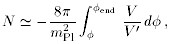
Hubble radius during inflation. The relevant number of e-foldings
from the end of inflation is given by
[2]
. We see that the amplitude of
perturbations depends on the
properties of the inflaton potential at the time the scale crossed the
Hubble radius during inflation. The relevant number of e-foldings
from the end of inflation is given by
[2]
 to be
substituted into Eqs. (55)
and (56).
to be
substituted into Eqs. (55)
and (56).
H2(k).
Back.