


6.3. Observational consequences
Observations have moved on beyond us wanting to know the overall normalization of the potential. The interesting things are
These can be neatly summarized using the slow-roll parameters
 and
and  we defined
earlier. [3]
we defined
earlier. [3]
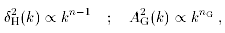
The standard approximation used to describe the spectra is the power-law approximation, where we take
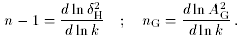
where the spectral indices n and nG are given by
The power-law approximation is usually valid because only a limited
range of scales are observable, with the range 1 Mpc to 104 Mpc
corresponding to
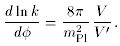
The crucial equation we need is that relating
(since within the slow-roll approximation
k
where now
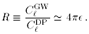
Finally, we need a measure of the relevant importance of density
perturbations and gravitational waves. The natural place to look is the
microwave background; a detailed calculation which I cannot reproduce here
(see e.g. Ref.
[2]) gives
Here the Cl are the contributions to the microwave
multipoles, in the usual notation.
(8)
From these expressions we immediately see
Table 1 shows the predictions for a range of inflation
models. The information I've given you so far should be sufficient to
allow you to reproduce them. Even the simplest inflation models can
affect the large-scale structure modelling at a level comparable to the
present observational accuracy. The predictions of the different models
will be wildly different as far as future high-accuracy observations are
concerned.
Observations have some way to go before the power-law approximation becomes
inadequate. Consequently ...
 ln k
ln k
 9.
9.
 values to when a scale
k crosses the Hubble radius, which from Eq. (58) is
values to when a scale
k crosses the Hubble radius, which from Eq. (58) is
 exp N). Direct
differentiation then yields
[3]
exp N). Direct
differentiation then yields
[3]
(62)

(63)
and
are to be evaluated
on the appropriate part of the potential.
<< 1 and
|| << 1 do we get
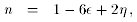
n 1 and
R 0.
is quite a bit smaller than one.
MODEL
POTENTIAL
n
R
Polynomial
2
0.97
0.1
chaotic inflation
4
0.95
0.2
Power-law inflation
exp(-  )
)
any n < 1
2  (1 - n)
`Natural' inflation
1 + cos( / f )
any n < 1
0
Hybrid inflation (standard)
1 + B 2
1
0
Hybrid inflation (extreme)
1 + B 2
1 < n < 1.15
~ 0
and
are the fundamental
parameters, it is
best to take them as n and R.
