


In our discussion of manifolds, it became clear that there were various notions we could talk about as soon as the manifold was defined; we could define functions, take their derivatives, consider parameterized paths, set up tensors, and so on. Other concepts, such as the volume of a region or the length of a path, required some additional piece of structure, namely the introduction of a metric. It would be natural to think of the notion of "curvature", which we have already used informally, is something that depends on the metric. Actually this turns out to be not quite true, or at least incomplete. In fact there is one additional structure we need to introduce - a "connection" - which is characterized by the curvature. We will show how the existence of a metric implies a certain connection, whose curvature may be thought of as that of the metric.
The connection becomes necessary when we attempt to address the
problem of the partial derivative not being a good tensor operator.
What we would like is a covariant derivative; that is, an operator
which reduces to the partial derivative in flat space with Cartesian
coordinates, but transforms as a tensor on an arbitrary manifold.
It is conventional to spend a certain amount of time motivating the
introduction of a covariant derivative, but in fact the need is
obvious; equations such as
![]() T
T![]()
![]() = 0 are going to have to
be generalized to curved space somehow. So let's agree that a
covariant derivative would be a good thing to have, and go about setting
it up.
= 0 are going to have to
be generalized to curved space somehow. So let's agree that a
covariant derivative would be a good thing to have, and go about setting
it up.
In flat space in Cartesian coordinates, the partial derivative operator
![]() is a map from (k, l ) tensor
fields to (k, l + 1) tensor fields,
which acts linearly on its arguments and obeys the Leibniz rule on
tensor products. All of this continues to be true in the more general
situation we would now like to consider, but the map provided by the
partial derivative depends on the coordinate system used.
We would therefore like to define a covariant derivative operator
is a map from (k, l ) tensor
fields to (k, l + 1) tensor fields,
which acts linearly on its arguments and obeys the Leibniz rule on
tensor products. All of this continues to be true in the more general
situation we would now like to consider, but the map provided by the
partial derivative depends on the coordinate system used.
We would therefore like to define a covariant derivative operator
![]() to perform the functions of the partial derivative, but
in a way independent of coordinates. We therefore require that
to perform the functions of the partial derivative, but
in a way independent of coordinates. We therefore require that
![]() be a map from (k, l ) tensor fields to
(k, l + 1) tensor fields
which has these two properties:
be a map from (k, l ) tensor fields to
(k, l + 1) tensor fields
which has these two properties:
If ![]() is going to obey the Leibniz rule, it can always be
written
as the partial derivative plus some linear transformation. That is,
to take the covariant derivative we first take the partial derivative,
and then apply a correction to make the result covariant. (We aren't
going to prove this reasonable-sounding statement, but Wald goes into
detail if you are interested.) Let's consider what this means for the
covariant derivative of a vector V
is going to obey the Leibniz rule, it can always be
written
as the partial derivative plus some linear transformation. That is,
to take the covariant derivative we first take the partial derivative,
and then apply a correction to make the result covariant. (We aren't
going to prove this reasonable-sounding statement, but Wald goes into
detail if you are interested.) Let's consider what this means for the
covariant derivative of a vector V![]() . It means that, for each
direction
. It means that, for each
direction ![]() , the covariant derivative
, the covariant derivative
![]() will be given
by the partial derivative
will be given
by the partial derivative
![]() plus a correction specified
by a matrix
(
plus a correction specified
by a matrix
(![]() )
)![]()
![]() (an n × n matrix,
where
n is the dimensionality of the manifold, for each
(an n × n matrix,
where
n is the dimensionality of the manifold, for each ![]() ). In fact
the parentheses are usually dropped and we write these matrices,
known as the connection coefficients, with haphazard index
placement as
). In fact
the parentheses are usually dropped and we write these matrices,
known as the connection coefficients, with haphazard index
placement as
![]() . We therefore have
. We therefore have
| (3.1) |
Notice that in the second term the index originally on V has moved
to the ![]() , and a new index is summed over. If this is the
expression for the covariant derivative of a vector in terms of the
partial derivative, we should be able to determine the transformation
properties of
, and a new index is summed over. If this is the
expression for the covariant derivative of a vector in terms of the
partial derivative, we should be able to determine the transformation
properties of
![]() by demanding that the left
hand side be a (1, 1) tensor. That is, we want the transformation
law to be
by demanding that the left
hand side be a (1, 1) tensor. That is, we want the transformation
law to be
| (3.2) |
Let's look at the left side first; we can expand it using (3.1) and then transform the parts that we understand:
| (3.3) |
The right side, meanwhile, can likewise be expanded:
| (3.4) |
These last two expressions are to be equated; the first terms in each are identical and therefore cancel, so we have
| (3.5) |
where we have changed a dummy index
from ![]() to
to ![]() . This equation must be true for any vector
V
. This equation must be true for any vector
V![]() , so we can eliminate that on both
sides. Then the
connection coefficients in the primed coordinates may be isolated by
multiplying by
, so we can eliminate that on both
sides. Then the
connection coefficients in the primed coordinates may be isolated by
multiplying by
![]() x
x![]() /
/![]() x
x![]() . The result
is
. The result
is
| (3.6) |
This is not, of course, the tensor transformation law; the second term
on the right spoils it. That's okay, because the connection
coefficients are not the components of a tensor. They are purposefully
constructed to be non-tensorial, but in such a way that the combination
(3.1) transforms as a tensor - the extra terms in the transformation
of the partials and the ![]() 's exactly cancel. This is why we
are not so careful about index placement on the connection coefficients;
they are not a tensor, and therefore you should try not to raise and
lower their indices.
's exactly cancel. This is why we
are not so careful about index placement on the connection coefficients;
they are not a tensor, and therefore you should try not to raise and
lower their indices.
What about the covariant derivatives of other sorts of tensors?
By similar reasoning to that used for vectors, the covariant
derivative of a one-form can also be expressed as a partial
derivative plus some linear transformation. But there is no reason
as yet that the matrices representing this transformation should be
related to the coefficients
![]() . In general
we could write something like
. In general
we could write something like
| (3.7) |
where
![]() is a new set of matrices
for each
is a new set of matrices
for each ![]() . (Pay attention to where all of the various indices go.)
It is straightforward to derive that the transformation properties
of
. (Pay attention to where all of the various indices go.)
It is straightforward to derive that the transformation properties
of
![]() must be the same as those of
must be the same as those of ![]() , but
otherwise no relationship has been established. To do so, we need to
introduce two new properties that we would like our covariant derivative
to have (in addition to the two above):
, but
otherwise no relationship has been established. To do so, we need to
introduce two new properties that we would like our covariant derivative
to have (in addition to the two above):
There is no way to "derive" these properties; we are simply demanding that they be true as part of the definition of a covariant derivative.
Let's see what these new properties imply. Given some one-form field
![]() and vector field V
and vector field V![]() , we can take the covariant
derivative of the scalar defined by
, we can take the covariant
derivative of the scalar defined by
![]() V
V![]() to
get
to
get
| (3.8) |
But since
![]() V
V![]() is a scalar, this must also
be given by the partial derivative:
is a scalar, this must also
be given by the partial derivative:
| (3.9) |
This can only be true if the terms in (3.8) with connection coefficients cancel each other; that is, rearranging dummy indices, we must have
| (3.10) |
But both
![]() and V
and V![]() are completely arbitrary,
so
are completely arbitrary,
so

| (3.11) |
The two extra conditions we have imposed therefore allow us to express the covariant derivative of a one-form using the same connection coefficients as were used for the vector, but now with a minus sign (and indices matched up somewhat differently):
| (3.12) |
It should come as no surprise that the connection coefficients
encode all of the information necessary to take the covariant
derivative of a tensor of arbitrary rank. The formula is quite
straightforward; for each upper index you introduce a term with
a single + ![]() , and for each lower index a term with a single
-
, and for each lower index a term with a single
- ![]() :
:
| (3.13) |
This is the general expression for the covariant derivative. You can check it yourself; it comes from the set of axioms we have established, and the usual requirements that tensors of various sorts be coordinate-independent entities. Sometimes an alternative notation is used; just as commas are used for partial derivatives, semicolons are used for covariant ones:

| (3.14) |
Once again, I'm not a big fan of this notation.
To define a covariant derivative, then, we need to put a
"connection" on our manifold, which is specified in some
coordinate system by a set of coefficients
![]() (n3 = 64 independent components in n = 4
dimensions) which transform according to (3.6).
(The name "connection" comes from the fact that it is used to
transport vectors from one tangent space to another, as we will
soon see.) There are evidently a large number of connections
we could define on any manifold, and each of them implies a
distinct notion of covariant differentiation. In general relativity
this freedom is not a big concern, because it turns out that every
metric defines a unique connection, which is the one used in GR.
Let's see how that works.
(n3 = 64 independent components in n = 4
dimensions) which transform according to (3.6).
(The name "connection" comes from the fact that it is used to
transport vectors from one tangent space to another, as we will
soon see.) There are evidently a large number of connections
we could define on any manifold, and each of them implies a
distinct notion of covariant differentiation. In general relativity
this freedom is not a big concern, because it turns out that every
metric defines a unique connection, which is the one used in GR.
Let's see how that works.
The first thing to notice is that the difference of two connections
is a (1, 2) tensor. If we have two sets of connection coefficients,
![]() and
and
![]() , their difference
S
, their difference
S![]()
![]()
![]() =
= ![]() -
- ![]() (notice
index placement) transforms as
(notice
index placement) transforms as
| (3.15) |
This is just the tensor transormation law, so
S![]()
![]()
![]() is
indeed a tensor. This implies that any set of connections can be
expressed as some fiducial connection plus a tensorial correction.
is
indeed a tensor. This implies that any set of connections can be
expressed as some fiducial connection plus a tensorial correction.
Next notice that, given a connection specified by
![]() ,
we can immediately form another connection simply by
permuting the lower indices. That is, the set of coefficients
,
we can immediately form another connection simply by
permuting the lower indices. That is, the set of coefficients
![]() will also transform according to (3.6)
(since the partial derivatives appearing in the last term can be
commuted), so they determine a distinct connection. There is thus
a tensor we can associate with any given connection, known as the
torsion tensor, defined by
will also transform according to (3.6)
(since the partial derivatives appearing in the last term can be
commuted), so they determine a distinct connection. There is thus
a tensor we can associate with any given connection, known as the
torsion tensor, defined by
| (3.16) |
It is clear that the torsion is antisymmetric its lower indices, and a connection which is symmetric in its lower indices is known as "torsion-free."
We can now define a unique connection on a manifold with a metric
g![]()
![]() by introducing two additional properties:
by introducing two additional properties:
A connection is metric compatible if the covariant derivative of the metric with respect to that connection is everywhere zero. This implies a couple of nice properties. First, it's easy to show that the inverse metric also has zero covariant derivative,

| (3.17) |
Second, a metric-compatible covariant derivative commutes with
raising and lowering of indices. Thus, for some vector field
V![]() ,
,
| (3.18) |
With non-metric-compatible connections one must be very careful about index placement when taking a covariant derivative.
Our claim is therefore that there is exactly one torsion-free connection on a given manifold which is compatible with some given metric on that manifold. We do not want to make these two requirements part of the definition of a covariant derivative; they simply single out one of the many possible ones.
We can demonstrate both existence and uniqueness by deriving a manifestly unique expression for the connection coefficients in terms of the metric. To accomplish this, we expand out the equation of metric compatibility for three different permutations of the indices:

| |
| (3.19) |
We subtract the second and third of these from the first, and use the symmetry of the connection to obtain

| (3.20) |
It is straightforward to solve this for the connection by multiplying
by g![]()
![]() . The result is
. The result is
| (3.21) |
This is one of the most important formulas in this subject; commit it to memory. Of course, we have only proved that if a metric-compatible and torsion-free connection exists, it must be of the form (3.21); you can check for yourself (for those of you without enough tedious computation in your lives) that the right hand side of (3.21) transforms like a connection.
This connection we have derived from the metric is the one on which
conventional general relativity is based (although we will keep an open
mind for a while longer). It is known by different names:
sometimes the Christoffel connection, sometimes the
Levi-Civita connection, sometimes the Riemannian connection.
The associated connection coefficients are sometimes called
Christoffel symbols and written as
![]()
![]()
![]()
![]()
![]() ; we will sometimes call them Christoffel symbols, but we
won't use the funny notation. The study of manifolds with metrics
and their associated connections is called "Riemannian geometry."
As far as I can tell the study of more general connections can be
traced back to Cartan, but I've never heard it called "Cartanian
geometry."
; we will sometimes call them Christoffel symbols, but we
won't use the funny notation. The study of manifolds with metrics
and their associated connections is called "Riemannian geometry."
As far as I can tell the study of more general connections can be
traced back to Cartan, but I've never heard it called "Cartanian
geometry."
Before putting our covariant derivatives to work, we should mention some miscellaneous properties. First, let's emphasize again that the connection does not have to be constructed from the metric. In ordinary flat space there is an implicit connection we use all the time - the Christoffel connection constructed from the flat metric. But we could, if we chose, use a different connection, while keeping the metric flat. Also notice that the coefficients of the Christoffel connection in flat space will vanish in Cartesian coordinates, but not in curvilinear coordinate systems. Consider for example the plane in polar coordinates, with metric
| (3.22) |
The nonzero components of the inverse metric are readily found to be
grr = 1 and
g![]()
![]() = r-2. (Notice
that we use r and
= r-2. (Notice
that we use r and ![]() as indices in an obvious notation.) We can compute
a typical connection coefficient:
as indices in an obvious notation.) We can compute
a typical connection coefficient:
| |
| (3.23) |
Sadly, it vanishes. But not all of them do:
| (3.24) |
Continuing to turn the crank, we eventually find
| (3.25) |
The existence of nonvanishing connection coefficients in curvilinear coordinate systems is the ultimate cause of the formulas for the divergence and so on that you find in books on electricity and magnetism.
Contrariwise, even in a curved space it is still possible to make the Christoffel symbols vanish at any one point. This is just because, as we saw in the last section, we can always make the first derivative of the metric vanish at a point; so by (3.21) the connection coefficients derived from this metric will also vanish. Of course this can only be established at a point, not in some neighborhood of the point.
Another useful property is that the formula for the divergence
of a vector (with respect to the Christoffel connection) has a
simplified form. The covariant divergence of V![]() is given by
is given by
| (3.26) |
It's easy to show (see pp. 106-108 of Weinberg) that the Christoffel connection satisfies
| (3.27) |
and we therefore obtain
| (3.28) |
There are also formulas for the divergences of higher-rank tensors, but they are generally not such a great simplification.
As the last factoid we should mention about connections, let us emphasize (once more) that the exterior derivative is a well-defined tensor in the absence of any connection. The reason this needs to be emphasized is that, if you happen to be using a symmetric (torsion-free) connection, the exterior derivative (defined to be the antisymmetrized partial derivative) happens to be equal to the antisymmetrized covariant derivative:
| (3.29) |
This has led some misfortunate souls to fret about the "ambiguity" of the exterior derivative in spaces with torsion, where the above simplification does not occur. There is no ambiguity: the exterior derivative does not involve the connection, no matter what connection you happen to be using, and therefore the torsion never enters the formula for the exterior derivative of anything.
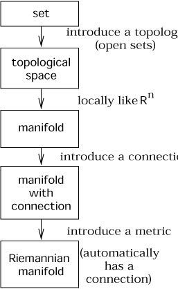
Before moving on, let's review the process by which we have been
adding structures to our mathematical constructs. We started with
the basic notion of a set, which you were presumed to know (informally,
if not rigorously). We introduced the concept of open subsets of
our set; this is equivalent
to introducing a topology, and promoted the set to a topological
space. Then by demanding that each open set look like a region of
![]() (with n the same for each set) and that
the coordinate
charts be smoothly sewn together, the topological space became a
manifold. A manifold is simultaneously a very flexible and powerful
structure, and comes equipped naturally with a tangent bundle,
tensor bundles of various ranks, the
ability to take exterior derivatives, and so forth. We then proceeded
to put a metric on the manifold, resulting in a manifold with metric
(or sometimes "Riemannian manifold").
Independently of the metric we found we could introduce a connection,
allowing us to take covariant derivatives. Once we have a metric,
however,
there is automatically a unique torsion-free metric-compatible
connection. (In principle there is nothing to stop us from introducing
more than one connection, or more than one metric, on any given
manifold.) The situation is thus as portrayed in the diagram on
the next page.
(with n the same for each set) and that
the coordinate
charts be smoothly sewn together, the topological space became a
manifold. A manifold is simultaneously a very flexible and powerful
structure, and comes equipped naturally with a tangent bundle,
tensor bundles of various ranks, the
ability to take exterior derivatives, and so forth. We then proceeded
to put a metric on the manifold, resulting in a manifold with metric
(or sometimes "Riemannian manifold").
Independently of the metric we found we could introduce a connection,
allowing us to take covariant derivatives. Once we have a metric,
however,
there is automatically a unique torsion-free metric-compatible
connection. (In principle there is nothing to stop us from introducing
more than one connection, or more than one metric, on any given
manifold.) The situation is thus as portrayed in the diagram on
the next page.
|
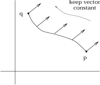
Having set up the machinery of connections, the first thing we will do is discuss parallel transport. Recall that in flat space it was unnecessary to be very careful about the fact that vectors were elements of tangent spaces defined at individual points; it is actually very natural to compare vectors at different points (where by "compare" we mean add, subtract, take the dot product, etc.). The reason why it is natural is because it makes sense, in flat space, to "move a vector from one point to another while keeping it constant." Then once we get the vector from one point to another we can do the usual operations allowed in a vector space.
|
The concept of moving a vector along a path, keeping constant all
the while, is known as parallel transport. As we shall see, parallel
transport is defined whenever we have a connection; the intuitive
manipulation of vectors in flat space makes implicit use of the
Christoffel connection on this space. The crucial difference between
flat and curved spaces is that, in a curved space, the result
of parallel transporting a vector from one point to another will
depend on the path taken between the points. Without yet assembling
the complete mechanism of parallel transport, we can use our
intuition about the two-sphere to see that this is the case. Start
with a vector on the equator, pointing along a line of constant
longitude. Parallel transport it up to the north pole along a line
of longitude in the
obvious way. Then take the original vector, parallel transport it
along the equator by an angle ![]() , and then move it up to the
north pole as before.
It is clear that the vector, parallel transported along two paths,
arrived at the same destination with two different values (rotated
by
, and then move it up to the
north pole as before.
It is clear that the vector, parallel transported along two paths,
arrived at the same destination with two different values (rotated
by ![]() ).
).

|
It therefore appears as if there is no natural way to uniquely move a vector from one tangent space to another; we can always parallel transport it, but the result depends on the path, and there is no natural choice of which path to take. Unlike some of the problems we have encountered, there is no solution to this one - we simply must learn to live with the fact that two vectors can only be compared in a natural way if they are elements of the same tangent space. For example, two particles passing by each other have a well-defined relative velocity (which cannot be greater than the speed of light). But two particles at different points on a curved manifold do not have any well-defined notion of relative velocity - the concept simply makes no sense. Of course, in certain special situations it is still useful to talk as if it did make sense, but it is necessary to understand that occasional usefulness is not a substitute for rigorous definition. In cosmology, for example, the light from distant galaxies is redshifted with respect to the frequencies we would observe from a nearby stationary source. Since this phenomenon bears such a close resemblance to the conventional Doppler effect due to relative motion, it is very tempting to say that the galaxies are "receding away from us" at a speed defined by their redshift. At a rigorous level this is nonsense, what Wittgenstein would call a "grammatical mistake" - the galaxies are not receding, since the notion of their velocity with respect to us is not well-defined. What is actually happening is that the metric of spacetime between us and the galaxies has changed (the universe has expanded) along the path of the photon from here to there, leading to an increase in the wavelength of the light. As an example of how you can go wrong, naive application of the Doppler formula to the redshift of galaxies implies that some of them are receding faster than light, in apparent contradiction with relativity. The resolution of this apparent paradox is simply that the very notion of their recession should not be taken literally.
Enough about what we cannot do; let's see what we can. Parallel
transport is supposed to be the curved-space generalization of the
concept of "keeping the vector constant" as we move it along
a path; similarly for a tensor of arbitrary rank. Given a
curve
x![]() (
(![]() ), the requirement of constancy of a tensor T
along this curve in flat space is simply
), the requirement of constancy of a tensor T
along this curve in flat space is simply
![]() =
= ![]()
![]() = 0.
We therefore define the covariant derivative along the path to be
given by an operator
= 0.
We therefore define the covariant derivative along the path to be
given by an operator

| (3.30) |
We then define parallel transport of the tensor T along
the path x![]() (
(![]() ) to be the requirement that, along the path,
) to be the requirement that, along the path,
| (3.31) |
This is a well-defined tensor equation, since both the tangent vector
dx![]() /d
/d![]() and the covariant derivative
and the covariant derivative ![]() T are tensors.
This is known as the equation of parallel transport. For
a vector it takes the form
T are tensors.
This is known as the equation of parallel transport. For
a vector it takes the form
| (3.32) |
We can look at the parallel transport equation as a first-order differential equation defining an initial-value problem: given a tensor at some point along the path, there will be a unique continuation of the tensor to other points along the path such that the continuation solves (3.31). We say that such a tensor is parallel transported.
The notion of parallel transport is obviously dependent on the connection, and different connections lead to different answers. If the connection is metric-compatible, the metric is always parallel transported with respect to it:
| (3.33) |
It follows that the inner product of two parallel-transported
vectors is preserved. That is, if V![]() and W
and W![]() are
parallel-transported along a curve x
are
parallel-transported along a curve x![]() (
(![]() ), we have
), we have
| (3.34) |
This means that parallel transport with respect to a metric-compatible connection preserves the norm of vectors, the sense of orthogonality, and so on.
One thing they don't usually tell you in GR books is that you can
write down an explicit and general solution to the parallel transport
equation, although it's somewhat formal. First notice that for some
path ![]() :
: ![]()
![]() x
x![]() (
(![]() ), solving the parallel
transport equation for a vector V
), solving the parallel
transport equation for a vector V![]() amounts to finding a matrix
P
amounts to finding a matrix
P![]()
![]() (
(![]() ,
,![]() ) which relates the vector at its
initial value
V
) which relates the vector at its
initial value
V![]() (
(![]() ) to its value somewhere later down the
path:
) to its value somewhere later down the
path:
| (3.35) |
Of course the matrix
P![]()
![]() (
(![]() ,
,![]() ), known as the
parallel propagator, depends on the
path
), known as the
parallel propagator, depends on the
path ![]() (although it's hard to find a notation which indicates
this without making
(although it's hard to find a notation which indicates
this without making ![]() look like an index). If we define
look like an index). If we define
| (3.36) |
where the quantities on the right hand side are evaluated at
x![]() (
(![]() ), then the parallel transport equation becomes
), then the parallel transport equation becomes
| (3.37) |
Since the parallel propagator must work for any vector, substituting
(3.35) into (3.37) shows that
P![]()
![]() (
(![]() ,
,![]() ) also obeys this equation:
) also obeys this equation:
| (3.38) |
To solve this equation, first integrate both sides:
| (3.39) |
The Kronecker delta, it is easy to see, provides the correct
normalization for
![]() =
= ![]() .
.
We can solve (3.39) by iteration, taking the right hand side and plugging it into itself repeatedly, giving

| (3.40) |
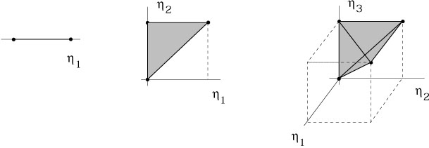
The nth term in this series is an integral over an n-dimensional right triangle, or n-simplex.

|
|
It would simplify things if we could consider such an integral to
be over an n-cube instead of an n-simplex; is there some way
to do this? There are n! such
simplices in each cube, so we would have to multiply by 1/n! to
compensate for this extra volume. But we also want to get the
integrand right; using matrix notation, the integrand at nth order
is A(![]() )A(
)A(![]() ) ... A(
) ... A(![]() ), but with the special
property that
), but with the special
property that
![]()
![]()
![]()
![]() ...
... ![]()
![]() .
We therefore define the path-ordering symbol,
.
We therefore define the path-ordering symbol, ![]() ,
to ensure that this condition holds. In other words, the expression
,
to ensure that this condition holds. In other words, the expression
| (3.41) |
stands for the product of the n matrices A(![]() ), ordered in
such a way that the largest value of
), ordered in
such a way that the largest value of ![]() is on the left, and
each subsequent value of
is on the left, and
each subsequent value of ![]() is less than or equal to the
previous one. We then can express the nth-order term in (3.40) as
is less than or equal to the
previous one. We then can express the nth-order term in (3.40) as
| (3.42) |
This expression contains no substantive statement about the matrices
A(![]() ); it is just notation. But we can now write
(3.40) in matrix form as
); it is just notation. But we can now write
(3.40) in matrix form as
| (3.43) |
This formula is just the series expression for an exponential; we therefore say that the parallel propagator is given by the path-ordered exponential
| (3.44) |
where once again this is just notation; the path-ordered exponential is defined to be the right hand side of (3.43). We can write it more explicitly as
| (3.45) |
It's nice to have an explicit formula, even if it is rather abstract. The same kind of expression appears in quantum field theory as "Dyson's Formula," where it arises because the Schrödinger equation for the time-evolution operator has the same form as (3.38).
As an aside, an especially interesting example of the parallel propagator occurs when the path is a loop, starting and ending at the same point. Then if the connection is metric-compatible, the resulting matrix will just be a Lorentz transformation on the tangent space at the point. This transformation is known as the "holonomy" of the loop. If you know the holonomy of every possible loop, that turns out to be equivalent to knowing the metric. This fact has let Ashtekar and his collaborators to examine general relativity in the "loop representation," where the fundamental variables are holonomies rather than the explicit metric. They have made some progress towards quantizing the theory in this approach, although the jury is still out about how much further progress can be made.
With parallel transport understood, the next logical step is to discuss geodesics. A geodesic is the curved-space generalization of the notion of a "straight line" in Euclidean space. We all know what a straight line is: it's the path of shortest distance between two points. But there is an equally good definition -- a straight line is a path which parallel transports its own tangent vector. On a manifold with an arbitrary (not necessarily Christoffel) connection, these two concepts do not quite coincide, and we should discuss them separately.
We'll take the second definition first, since it is computationally
much more straightforward. The tangent vector to a path
x![]() (
(![]() ) is
dx
) is
dx![]() /d
/d![]() . The condition that it be parallel transported
is thus
. The condition that it be parallel transported
is thus

| (3.46) |
or alternatively
| (3.47) |
This is the geodesic equation, another one which you should
memorize. We can easily see that it reproduces the usual notion
of straight lines if the connection coefficients are the Christoffel
symbols in Euclidean space; in that case we can choose Cartesian
coordinates in which
![]() = 0, and the geodesic
equation is just
d2x
= 0, and the geodesic
equation is just
d2x![]() /d
/d![]() = 0, which is the equation for
a straight line.
= 0, which is the equation for
a straight line.
That was embarrassingly simple; let's turn to the more nontrivial case of the shortest distance definition. As we know, there are various subtleties involved in the definition of distance in a Lorentzian spacetime; for null paths the distance is zero, for timelike paths it's more convenient to use the proper time, etc. So in the name of simplicity let's do the calculation just for a timelike path - the resulting equation will turn out to be good for any path, so we are not losing any generality. We therefore consider the proper time functional,
| (3.48) |
where the integral is over the path. To search for shortest-distance paths, we will do the usual calculus of variations treatment to seek extrema of this functional. (In fact they will turn out to be curves of maximum proper time.)
We want to consider the change in the proper time under infinitesimal variations of the path,
| (3.49) |
(The second line comes from Taylor expansion in curved spacetime, which as you can see uses the partial derivative, not the covariant derivative.) Plugging this into (3.48), we get
| (3.50) |
Since
![]() x
x![]() is assumed to be small, we can
expand the
square root of the expression in square brackets to find
is assumed to be small, we can
expand the
square root of the expression in square brackets to find

| (3.51) |
It is helpful at this point to change the parameterization of our
curve from ![]() , which was arbitrary, to the proper time
, which was arbitrary, to the proper time ![]() itself, using
itself, using
| (3.52) |
We plug this into (3.51) (note: we plug it in for every appearance
of d![]() ) to obtain
) to obtain
| |
| (3.53) |
where in the last line we have integrated by parts, avoiding possible
boundary contributions by demanding that the variation
![]() x
x![]() vanish at the endpoints of the path. Since we are searching for
stationary points, we want
vanish at the endpoints of the path. Since we are searching for
stationary points, we want
![]()
![]() to vanish for any variation;
this implies
to vanish for any variation;
this implies
| (3.54) |
where we have used dg![]()
![]() /d
/d![]() = (dx
= (dx![]() /d
/d![]() )
)![]() g
g![]()
![]() . Some shuffling of dummy indices
reveals
. Some shuffling of dummy indices
reveals
| (3.55) |
and multiplying by the inverse metric finally leads to
| (3.56) |
We see that this is precisely the geodesic equation (3.32), but with the specific choice of Christoffel connection (3.21). Thus, on a manifold with metric, extremals of the length functional are curves which parallel transport their tangent vector with respect to the Christoffel connection associated with that metric. It doesn't matter if there is any other connection defined on the same manifold. Of course, in GR the Christoffel connection is the only one which is used, so the two notions are the same.
The primary usefulness of geodesics in general relativity is that
they are the paths followed by unaccelerated particles. In fact,
the geodesic equation can be thought of as the generalization of
Newton's law
![]() = m
= m![]() for the case
for the case ![]() = 0. It is
also possible to introduce forces by adding terms to the right hand
side; in fact, looking back to the expression (1.103) for the
Lorentz force in special relativity, it is tempting to guess that
the equation of motion for a particle of mass m and charge q
in general relativity should be
= 0. It is
also possible to introduce forces by adding terms to the right hand
side; in fact, looking back to the expression (1.103) for the
Lorentz force in special relativity, it is tempting to guess that
the equation of motion for a particle of mass m and charge q
in general relativity should be
| (3.57) |
We will talk about this more later, but in fact your guess would be correct.
Having boldly derived these expressions, we should say some more
careful words about the parameterization of a geodesic path.
When we presented the geodesic equation as the requirement that
the tangent vector be parallel transported, (3.47), we parameterized
our path with some parameter ![]() , whereas when we found
the formula (3.56) for the extremal of the spacetime interval we wound
up with a very specific parameterization, the proper time. Of course
from the form of (3.56) it is clear that a transformation
, whereas when we found
the formula (3.56) for the extremal of the spacetime interval we wound
up with a very specific parameterization, the proper time. Of course
from the form of (3.56) it is clear that a transformation
| (3.58) |
for some constants a and b, leaves the equation invariant. Any parameter related to the proper time in this way is called an affine parameter, and is just as good as the proper time for parameterizing a geodesic. What was hidden in our derivation of (3.47) was that the demand that the tangent vector be parallel transported actually constrains the parameterization of the curve, specifically to one related to the proper time by (3.58). In other words, if you start at some point and with some initial direction, and then construct a curve by beginning to walk in that direction and keeping your tangent vector parallel transported, you will not only define a path in the manifold but also (up to linear transformations) define the parameter along the path.
Of course, there is nothing to stop you from using any other parameterization you like, but then (3.47) will not be satisfied. More generally you will satisfy an equation of the form
| (3.59) |
for some parameter ![]() and some function f (
and some function f (![]() ).
Conversely, if (3.59) is satisfied along a curve you can always find
an affine parameter
).
Conversely, if (3.59) is satisfied along a curve you can always find
an affine parameter
![]() (
(![]() ) for which the geodesic equation
(3.47) will be satisfied.
) for which the geodesic equation
(3.47) will be satisfied.
An important property of geodesics in a spacetime with Lorentzian metric is that the character (timelike/null/spacelike) of the geodesic (relative to a metric-compatible connection) never changes. This is simply because parallel transport preserves inner products, and the character is determined by the inner product of the tangent vector with itself. This is why we were consistent to consider purely timelike paths when we derived (3.56); for spacelike paths we would have derived the same equation, since the only difference is an overall minus sign in the final answer. There are also null geodesics, which satisfy the same equation, except that the proper time cannot be used as a parameter (some set of allowed parameters will exist, related to each other by linear transformations). You can derive this fact either from the simple requirement that the tangent vector be parallel transported, or by extending the variation of (3.48) to include all non-spacelike paths.
Let's now explain the earlier remark that timelike geodesics are maxima of the proper time. The reason we know this is true is that, given any timelike curve (geodesic or not), we can approximate it to arbitrary accuracy by a null curve. To do this all we have to do is to consider "jagged" null curves which follow the timelike one:

|
As we increase the number of sharp corners, the null curve comes closer and closer to the timelike curve while still having zero path length. Timelike geodesics cannot therefore be curves of minimum proper time, since they are always infinitesimally close to curves of zero proper time; in fact they maximize the proper time. (This is how you can remember which twin in the twin paradox ages more - the one who stays home is basically on a geodesic, and therefore experiences more proper time.) Of course even this is being a little cavalier; actually every time we say "maximize" or "minimize" we should add the modifier "locally." It is often the case that between two points on a manifold there is more than one geodesic. For instance, on S2 we can draw a great circle through any two points, and imagine travelling between them either the short way or the long way around. One of these is obviously longer than the other, although both are stationary points of the length functional.
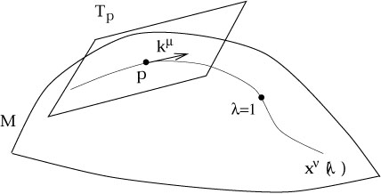
The final fact about geodesics before we move on to curvature proper
is their use in mapping the tangent space at a point p to a local
neighborhood of p. To do this we notice that any geodesic
x![]() (
(![]() ) which passes through p can be specified by its
behavior at p; let us choose the parameter value to be
) which passes through p can be specified by its
behavior at p; let us choose the parameter value to be
![]() (p) = 0, and the tangent vector at p to
be
(p) = 0, and the tangent vector at p to
be
| (3.60) |
for k![]() some vector at p (some element
of Tp). Then
there will be a unique point on the manifold M which lies on
this geodesic where the
parameter has the value
some vector at p (some element
of Tp). Then
there will be a unique point on the manifold M which lies on
this geodesic where the
parameter has the value ![]() = 1. We define the exponential
map at p,
expp : Tp
= 1. We define the exponential
map at p,
expp : Tp ![]() M, via
M, via
| (3.61) |
where x![]() (
(![]() ) solves the geodesic equation subject to (3.60).
) solves the geodesic equation subject to (3.60).
|
For some set of tangent vectors k![]() near the zero vector,
this map will be well-defined, and in fact invertible. Thus in the
neighborhood of p given by the range of the map on this set of
tangent vectors, the the tangent vectors themselves define a coordinate
system on the manifold. In this coordinate system, any geodesic
through p is expressed trivially as
near the zero vector,
this map will be well-defined, and in fact invertible. Thus in the
neighborhood of p given by the range of the map on this set of
tangent vectors, the the tangent vectors themselves define a coordinate
system on the manifold. In this coordinate system, any geodesic
through p is expressed trivially as

| (3.62) |
for some appropriate vector k![]() .
.
We won't go into detail about the properties of the exponential map, since in fact we won't be using it much, but it's important to emphasize that the range of the map is not necessarily the whole manifold, and the domain is not necessarily the whole tangent space. The range can fail to be all of M simply because there can be two points which are not connected by any geodesic. (In a Euclidean signature metric this is impossible, but not in a Lorentzian spacetime.) The domain can fail to be all of Tp because a geodesic may run into a singularity, which we think of as "the edge of the manifold." Manifolds which have such singularities are known as geodesically incomplete. This is not merely a problem for careful mathematicians; in fact the "singularity theorems" of Hawking and Penrose state that, for reasonable matter content (no negative energies), spacetimes in general relativity are almost guaranteed to be geodesically incomplete. As examples, the two most useful spacetimes in GR - the Schwarzschild solution describing black holes and the Friedmann-Robertson-Walker solutions describing homogeneous, isotropic cosmologies - both feature important singularities.
Having set up the machinery of parallel transport and covariant derivatives, we are at last prepared to discuss curvature proper. The curvature is quantified by the Riemann tensor, which is derived from the connection. The idea behind this measure of curvature is that we know what we mean by "flatness" of a connection - the conventional (and usually implicit) Christoffel connection associated with a Euclidean or Minkowskian metric has a number of properties which can be thought of as different manifestations of flatness. These include the fact that parallel transport around a closed loop leaves a vector unchanged, that covariant derivatives of tensors commute, and that initially parallel geodesics remain parallel. As we shall see, the Riemann tensor arises when we study how any of these properties are altered in more general contexts.
We have already argued, using the two-sphere as an example, that parallel
transport of a vector around a closed loop in a curved space will lead
to a transformation of the vector. The resulting transformation
depends on the total curvature enclosed by the loop; it would be more
useful to have a local description of the curvature at each point,
which is what the Riemann tensor is supposed to provide.
One conventional way to introduce the Riemann tensor, therefore,
is to consider parallel transport around an
infinitesimal loop. We are not going to do that here, but take a
more direct route. (Most of the presentations in the literature are
either sloppy, or correct but very difficult to follow.) Nevertheless,
even without working through the details, it is possible to see what
form the answer should take. Imagine that we parallel transport a
vector V![]() around a closed loop defined by two
vectors A
around a closed loop defined by two
vectors A![]() and
B
and
B![]() :
:

|
The (infinitesimal) lengths of the sides of the loop are ![]() a and
a and ![]() b, respectively. Now, we know the action of parallel
transport is independent of coordinates, so there should be some
tensor which tells us how the vector changes when it comes back to
its starting point; it will be a linear transformation on a vector,
and therefore involve one upper and one lower index. But it will
also depend on the two vectors A and B which define the loop;
therefore there should be two additional lower indices to contract with
A
b, respectively. Now, we know the action of parallel
transport is independent of coordinates, so there should be some
tensor which tells us how the vector changes when it comes back to
its starting point; it will be a linear transformation on a vector,
and therefore involve one upper and one lower index. But it will
also depend on the two vectors A and B which define the loop;
therefore there should be two additional lower indices to contract with
A![]() and B
and B![]() . Furthermore, the tensor should be
antisymmetric
in these two indices, since interchanging the vectors corresponds to
traversing the loop in the opposite direction, and should give the
inverse of the original answer. (This is consistent with the
fact that the transformation should vanish if A and B
are the same vector.) We therefore expect that the expression for
the change
. Furthermore, the tensor should be
antisymmetric
in these two indices, since interchanging the vectors corresponds to
traversing the loop in the opposite direction, and should give the
inverse of the original answer. (This is consistent with the
fact that the transformation should vanish if A and B
are the same vector.) We therefore expect that the expression for
the change
![]() V
V![]() experienced by this vector when parallel
transported around the loop should be of the form
experienced by this vector when parallel
transported around the loop should be of the form

| (3.63) |
where
R![]()
![]()
![]()
![]() is a (1, 3) tensor known as the
Riemann tensor (or simply "curvature tensor"). It is
antisymmetric in the last two indices:
is a (1, 3) tensor known as the
Riemann tensor (or simply "curvature tensor"). It is
antisymmetric in the last two indices:
| (3.64) |
(Of course, if (3.63) is taken as a definition of the Riemann tensor, there is a convention that needs to be chosen for the ordering of the indices. There is no agreement at all on what this convention should be, so be careful.)
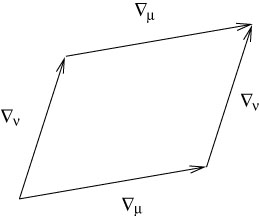
Knowing what we do about parallel transport, we could very carefully perform the necessary manipulations to see what happens to the vector under this operation, and the result would be a formula for the curvature tensor in terms of the connection coefficients. It is much quicker, however, to consider a related operation, the commutator of two covariant derivatives. The relationship between this and parallel transport around a loop should be evident; the covariant derivative of a tensor in a certain direction measures how much the tensor changes relative to what it would have been if it had been parallel transported (since the covariant derivative of a tensor in a direction along which it is parallel transported is zero). The commutator of two covariant derivatives, then, measures the difference between parallel transporting the tensor first one way and then the other, versus the opposite ordering.
|
The actual computation is very straightforward. Considering a
vector field V![]() , we take
, we take
| (3.65) |
In the last step we have relabeled some dummy indices and eliminated some terms that cancel when antisymmetrized. We recognize that the last term is simply the torsion tensor, and that the left hand side is manifestly a tensor; therefore the expression in parentheses must be a tensor itself. We write

| (3.66) |
where the Riemann tensor is identified as

| (3.67) |
There are a number of things to notice about the derivation of this expression:
| (3.68) |
A useful notion is that of the commutator of two vector fields X and Y, which is a third vector field with components
| (3.69) |
Both the torsion tensor and the Riemann tensor, thought of as multilinear maps, have elegant expressions in terms of the commutator. Thinking of the torsion as a map from two vector fields to a third vector field, we have

| (3.70) |
and thinking of the Riemann tensor as a map from three vector fields to a fourth one, we have

| (3.71) |
In these expressions, the notation ![]() refers to the covariant
derivative along the vector field X; in components,
refers to the covariant
derivative along the vector field X; in components,
![]() = X
= X![]()
![]() . Note that the two vectors X and
Y in (3.71)
correspond to the two antisymmetric indices in the component form
of the Riemann tensor. The last term in (3.71), involving the
commutator [X, Y], vanishes when X and Y are
taken to be the coordinate basis vector fields (since
[
. Note that the two vectors X and
Y in (3.71)
correspond to the two antisymmetric indices in the component form
of the Riemann tensor. The last term in (3.71), involving the
commutator [X, Y], vanishes when X and Y are
taken to be the coordinate basis vector fields (since
[![]() ,
,![]() ] = 0), which
is why this term did not arise when we originally took the commutator
of two covariant derivatives. We will not use this notation
extensively, but you might see it in the literature, so you should
be able to decode it.
] = 0), which
is why this term did not arise when we originally took the commutator
of two covariant derivatives. We will not use this notation
extensively, but you might see it in the literature, so you should
be able to decode it.
Having defined the curvature tensor as something which characterizes the connection, let us now admit that in GR we are most concerned with the Christoffel connection. In this case the connection is derived from the metric, and the associated curvature may be thought of as that of the metric itself. This identification allows us to finally make sense of our informal notion that spaces for which the metric looks Euclidean or Minkowskian are flat. In fact it works both ways: if the components of the metric are constant in some coordinate system, the Riemann tensor will vanish, while if the Riemann tensor vanishes we can always construct a coordinate system in which the metric components are constant.
The first of these is easy to show. If we are in some coordinate system
such that
![]() g
g![]()
![]() = 0 (everywhere, not just at a point),
then
= 0 (everywhere, not just at a point),
then
![]() = 0 and
= 0 and
![]()
![]() = 0; thus
R
= 0; thus
R![]()
![]()
![]()
![]() = 0 by (3.67). But this is a tensor
equation, and
if it is true in one coordinate system it must be true in any coordinate
system. Therefore, the statement that the Riemann tensor vanishes
is a necessary condition for it to be possible to find coordinates in
which the components of
g
= 0 by (3.67). But this is a tensor
equation, and
if it is true in one coordinate system it must be true in any coordinate
system. Therefore, the statement that the Riemann tensor vanishes
is a necessary condition for it to be possible to find coordinates in
which the components of
g![]()
![]() are constant everywhere.
are constant everywhere.
It is also a sufficient condition, although we have to work harder to
show it. Start by choosing Riemann normal coordinates at some point
p, so that
g![]()
![]() =
= ![]() at p. (Here we are using
at p. (Here we are using
![]() in a generalized sense, as a matrix with either +1 or -1 for each
diagonal element and zeroes elsewhere. The actual arrangement of
the +1's and -1's depends on the canonical form of the metric, but
is irrelevant for the present argument.) Denote the basis vectors at
p by
in a generalized sense, as a matrix with either +1 or -1 for each
diagonal element and zeroes elsewhere. The actual arrangement of
the +1's and -1's depends on the canonical form of the metric, but
is irrelevant for the present argument.) Denote the basis vectors at
p by
![]() , with components
, with components
![]() . Then by construction
we have
. Then by construction
we have
| (3.72) |
Now let us parallel transport the entire set of basis vectors from p to another point q; the vanishing of the Riemann tensor ensures that the result will be independent of the path taken between p and q. Since parallel transport with respect to a metric compatible connection preserves inner products, we must have
| (3.73) |
We therefore have specified a set of vector fields which
everywhere define a basis in which the metric components are constant.
This is completely unimpressive; it can be done on any manifold,
regardless of what the curvature is. What we would like to show
is that this is a coordinate basis (which can only be true
if the curvature vanishes).
We know that if the
![]() 's are a coordinate basis, their
commutator will vanish:
's are a coordinate basis, their
commutator will vanish:

| (3.74) |
What we would really like is the converse: that if the commutator
vanishes we can find coordinates y![]() such that
such that
![]() =
= ![]() . In fact this is a true result, known as
Frobenius's Theorem. It's something of a mess to prove, involving
a good deal more mathematical apparatus than we have bothered to set
up. Let's just take it for granted (skeptics can consult Schutz's
Geometrical Methods book). Thus, we would like to demonstrate
(3.74) for the vector fields we have set up. Let's use the expression
(3.70) for the torsion:
. In fact this is a true result, known as
Frobenius's Theorem. It's something of a mess to prove, involving
a good deal more mathematical apparatus than we have bothered to set
up. Let's just take it for granted (skeptics can consult Schutz's
Geometrical Methods book). Thus, we would like to demonstrate
(3.74) for the vector fields we have set up. Let's use the expression
(3.70) for the torsion:

| (3.75) |
The torsion vanishes by hypothesis. The covariant derivatives will
also vanish, given the method by which we constructed our vector fields;
they were made by parallel transporting along arbitrary paths. If the
fields are parallel transported along arbitrary paths, they are
certainly parallel transported along the vectors
![]() , and therefore
their covariant derivatives in the direction of these vectors will
vanish. Thus (3.70) implies that the commutator vanishes, and therefore
that we can find a coordinate system y
, and therefore
their covariant derivatives in the direction of these vectors will
vanish. Thus (3.70) implies that the commutator vanishes, and therefore
that we can find a coordinate system y![]() for which these vector
fields are the partial derivatives. In this coordinate system the
metric will have components
for which these vector
fields are the partial derivatives. In this coordinate system the
metric will have components
![]() , as desired.
, as desired.
The Riemann tensor, with four indices, naively has n4 independent components in an n-dimensional space. In fact the antisymmetry property (3.64) means that there are only n(n - 1)/2 independent values these last two indices can take on, leaving us with n3(n - 1)/2 independent components. When we consider the Christoffel connection, however, there are a number of other symmetries that reduce the independent components further. Let's consider these now.
The simplest way to derive these additional symmetries is to examine the Riemann tensor with all lower indices,
| (3.76) |
Let us further consider the components of this tensor in Riemann normal coordinates established at a point p. Then the Christoffel symbols themselves will vanish, although their derivatives will not. We therefore have
| |
| (3.77) |
In the second line we have used
![]() g
g![]()
![]() = 0
in RNC's, and in the third line the fact that partials commute.
From this expression we can notice immediately two properties
of
R
= 0
in RNC's, and in the third line the fact that partials commute.
From this expression we can notice immediately two properties
of
R![]()
![]()
![]()
![]() ; it is antisymmetric in its first two
indices,
; it is antisymmetric in its first two
indices,
| (3.78) |
and it is invariant under interchange of the first pair of indices with the second:

| (3.79) |
With a little more work, which we leave to your imagination, we can see that the sum of cyclic permutations of the last three indices vanishes:
| (3.80) |
This last property is equivalent to the vanishing of the antisymmetric part of the last three indices:

| (3.81) |
All of these properties have been derived in a special coordinate system, but they are all tensor equations; therefore they will be true in any coordinates. Not all of them are independent; with some effort, you can show that (3.64), (3.78) and (3.81) together imply (3.79). The logical interdependence of the equations is usually less important than the simple fact that they are true.
Given these relationships between the different components of the
Riemann tensor, how many independent quantities remain? Let's
begin with the facts that R![]()
![]()
![]()
![]() is antisymmetric
in the first two indices, antisymmetric in the last two indices,
and symmetric under interchange of these two pairs. This means that
we can think of it as a symmetric matrix
R[
is antisymmetric
in the first two indices, antisymmetric in the last two indices,
and symmetric under interchange of these two pairs. This means that
we can think of it as a symmetric matrix
R[![]()
![]() ][
][![]()
![]() ],
where the pairs
],
where the pairs
![]()
![]() and
and ![]()
![]() are thought of as individual
indices. An m × m symmetric matrix has
m(m + 1)/2 independent
components, while an n × n antisymmetric matrix has
n(n - 1)/2
independent components. We therefore have
are thought of as individual
indices. An m × m symmetric matrix has
m(m + 1)/2 independent
components, while an n × n antisymmetric matrix has
n(n - 1)/2
independent components. We therefore have
| (3.82) |
independent components. We still have to deal with the additional symmetry (3.81). An immediate consequence of (3.81) is that the totally antisymmetric part of the Riemann tensor vanishes,

| (3.83) |
In fact, this equation plus the other symmetries (3.64), (3.78) and (3.79) are enough to imply (3.81), as can be easily shown by expanding (3.83) and messing with the resulting terms. Therefore imposing the additional constraint of (3.83) is equivalent to imposing (3.81), once the other symmetries have been accounted for. How many independent restrictions does this represent? Let us imagine decomposing
| (3.84) |
It is easy to see that any totally antisymmetric 4-index tensor
is automatically antisymmetric in its first and last indices, and
symmetric under interchange of the two pairs. Therefore these
properties are independent restrictions on
X![]()
![]()
![]()
![]() ,
unrelated to the requirement (3.83). Now a
totally antisymmetric 4-index tensor has
n(n - 1)(n - 2)(n - 3)/4!
terms, and therefore (3.83) reduces the number of independent
components by this amount. We are left with
,
unrelated to the requirement (3.83). Now a
totally antisymmetric 4-index tensor has
n(n - 1)(n - 2)(n - 3)/4!
terms, and therefore (3.83) reduces the number of independent
components by this amount. We are left with

| (3.85) |
independent components of the Riemann tensor.
In four dimensions, therefore, the Riemann tensor has 20 independent components. (In one dimension it has none.) These twenty functions are precisely the 20 degrees of freedom in the second derivatives of the metric which we could not set to zero by a clever choice of coordinates. This should reinforce your confidence that the Riemann tensor is an appropriate measure of curvature.
In addition to the algebraic symmetries of the Riemann tensor (which constrain the number of independent components at any point), there is a differential identity which it obeys (which constrains its relative values at different points). Consider the covariant derivative of the Riemann tensor, evaluated in Riemann normal coordinates:
| (3.86) |
We would like to consider the sum of cyclic permutations of the first three indices:
| (3.87) |
Once again, since this is an equation between tensors it is true in any
coordinate system, even though we derived it in a particular one.
We recognize by now that the antisymmetry R![]()
![]()
![]()
![]() = - R
= - R![]()
![]()
![]()
![]() allows us to write this result as
allows us to write this result as

| (3.88) |
This is known as the Bianchi identity. (Notice that for a general connection there would be additional terms involving the torsion tensor.) It is closely related to the Jacobi identity, since (as you can show) it basically expresses

| (3.89) |
It is frequently useful to consider contractions of the Riemann tensor. Even without the metric, we can form a contraction known as the Ricci tensor:

| (3.90) |
Notice that, for the curvature tensor formed from an arbitrary (not necessarily Christoffel) connection, there are a number of independent contractions to take. Our primary concern is with the Christoffel connection, for which (3.90) is the only independent contraction (modulo conventions for the sign, which of course change from place to place). The Ricci tensor associated with the Christoffel connection is symmetric,

| (3.91) |
as a consequence of the various symmetries of the Riemann tensor. Using the metric, we can take a further contraction to form the Ricci scalar:
| (3.92) |
An especially useful form of the Bianchi identity comes from contracting twice on (3.87):
| (3.93) |
or
| (3.94) |
(Notice that, unlike the partial derivative, it makes sense to raise an index on the covariant derivative, due to metric compatibility.) If we define the Einstein tensor as
| (3.95) |
then we see that the twice-contracted Bianchi identity (3.94) is equivalent to

| (3.96) |
The Einstein tensor, which is symmetric due to the symmetry of the Ricci tensor and the metric, will be of great importance in general relativity.
The Ricci tensor and the Ricci scalar contain information about "traces" of the Riemann tensor. It is sometimes useful to consider separately those pieces of the Riemann tensor which the Ricci tensor doesn't tell us about. We therefore invent the Weyl tensor, which is basically the Riemann tensor with all of its contractions removed. It is given in n dimensions by

| (3.97) |
This messy formula is designed so that all possible contractions of
C![]()
![]()
![]()
![]() vanish, while it retains the symmetries
of the Riemann tensor:
vanish, while it retains the symmetries
of the Riemann tensor:
| (3.98) |
The Weyl tensor is only defined in three or more dimensions, and
in three dimensions it vanishes identically. For n ![]() 4 it
satisfies a version of the Bianchi identity,
4 it
satisfies a version of the Bianchi identity,
| (3.99) |
One of the most important properties of the Weyl tensor is that
it is invariant under conformal transformations. This means that
if you compute
C![]()
![]()
![]()
![]() for some metric
g
for some metric
g![]()
![]() , and
then compute it again for a metric given by
, and
then compute it again for a metric given by
![]() (x)g
(x)g![]()
![]() ,
where
,
where ![]() (x) is an arbitrary nonvanishing function of
spacetime, you get the same answer. For this reason it is often
known as the "conformal tensor."
(x) is an arbitrary nonvanishing function of
spacetime, you get the same answer. For this reason it is often
known as the "conformal tensor."
After this large amount of formalism, it might be time to step back and think about what curvature means for some simple examples. First notice that, according to (3.85), in 1, 2, 3 and 4 dimensions there are 0, 1, 6 and 20 components of the curvature tensor, respectively. (Everything we say about the curvature in these examples refers to the curvature associated with the Christoffel connection, and therefore the metric.) This means that one-dimensional manifolds (such as S1) are never curved; the intuition you have that tells you that a circle is curved comes from thinking of it embedded in a certain flat two-dimensional plane. (There is something called "extrinsic curvature," which characterizes the way something is embedded in a higher dimensional space. Our notion of curvature is "intrinsic," and has nothing to do with such embeddings.)
The distinction between intrinsic and extrinsic curvature is also
important in two dimensions, where the curvature has one independent
component. (In fact, all of the information about the curvature is
contained in the single component of the Ricci scalar.) Consider
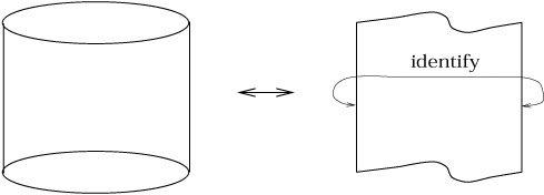
a cylinder,
![]() × S1.
× S1.
|
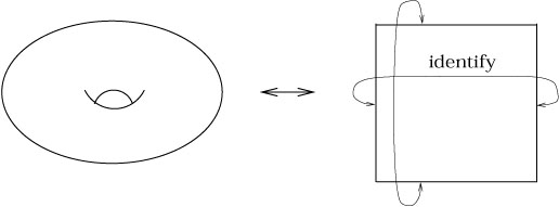
Although this looks curved from our point of view, it should be clear that we can put a metric on the cylinder whose components are constant in an appropriate coordinate system -- simply unroll it and use the induced metric from the plane. In this metric, the cylinder is flat. (There is also nothing to stop us from introducing a different metric in which the cylinder is not flat, but the point we are trying to emphasize is that it can be made flat in some metric.) The same story holds for the torus:
|
We can think of the torus as a square region of the plane with opposite sides identified (in other words, S1 × S1), from which it is clear that it can have a flat metric even though it looks curved from the embedded point of view.
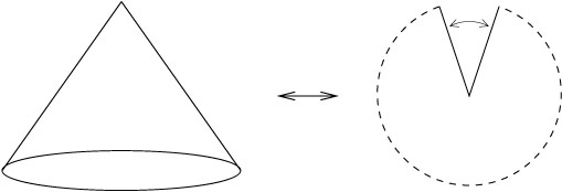
A cone is an example of a two-dimensional manifold with nonzero curvature at exactly one point. We can see this also by unrolling it; the cone is equivalent to the plane with a "deficit angle" removed and opposite sides identified:
|
In the metric inherited from this description as part of the flat plane, the cone is flat everywhere but at its vertex. This can be seen by considering parallel transport of a vector around various loops; if a loop does not enclose the vertex, there will be no overall transformation, whereas a loop that does enclose the vertex (say, just one time) will lead to a rotation by an angle which is just the deficit angle.
|
Our favorite example is of course the two-sphere, with metric
| (3.100) |
where a is the radius of the sphere (thought of as embedded in
![]() ). Without going through the details, the nonzero
connection coefficients are
). Without going through the details, the nonzero
connection coefficients are
| (3.101) |
Let's compute a promising component of the Riemann tensor:

| |
| (3.102) |
(The notation is obviously imperfect, since the Greek letter ![]() is a dummy index which is summed over, while the Greek letters
is a dummy index which is summed over, while the Greek letters
![]() and
and ![]() represent specific coordinates.) Lowering an
index, we have
represent specific coordinates.) Lowering an
index, we have
| (3.103) |
It is easy to check that all of the components of the Riemann tensor
either vanish or are related to this one by symmetry. We can go on
to compute the Ricci tensor via
R![]()
![]() = g
= g![]()
![]() R
R![]()
![]()
![]()
![]() . We obtain
. We obtain
| (3.104) |
The Ricci scalar is similarly straightforward:
| (3.105) |
Therefore the Ricci scalar, which for a two-dimensional manifold completely characterizes the curvature, is a constant over this two-sphere. This is a reflection of the fact that the manifold is "maximally symmetric," a concept we will define more precisely later (although it means what you think it should). In any number of dimensions the curvature of a maximally symmetric space satisfies (for some constant a)
| (3.106) |
which you may check is satisfied by this example.
Notice that the Ricci scalar is not only constant for the two-sphere, it is manifestly positive. We say that the sphere is "positively curved" (of course a convention or two came into play, but fortunately our conventions conspired so that spaces which everyone agrees to call positively curved actually have a positive Ricci scalar). From the point of view of someone living on a manifold which is embedded in a higher-dimensional Euclidean space, if they are sitting at a point of positive curvature the space curves away from them in the same way in any direction, while in a negatively curved space it curves away in opposite directions. Negatively curved spaces are therefore saddle-like.

|
Enough fun with examples. There is one more topic we have to cover before introducing general relativity itself: geodesic deviation. You have undoubtedly heard that the defining property of Euclidean (flat) geometry is the parallel postulate: initially parallel lines remain parallel forever. Of course in a curved space this is not true; on a sphere, certainly, initially parallel geodesics will eventually cross. We would like to quantify this behavior for an arbitrary curved space.
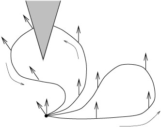
The problem is that the notion of "parallel" does not extend
naturally from flat to curved spaces. Instead what we will do is
to construct a one-parameter family of geodesics,
![]() (t).
That is, for each
s
(t).
That is, for each
s ![]()
![]() ,
, ![]() is a geodesic parameterized
by the affine parameter t.
The collection of these curves defines a smooth two-dimensional
surface (embedded in a manifold M of arbitrary dimensionality). The
coordinates on this surface may be chosen to be s and t,
provided
we have chosen a family of geodesics which do not cross. The entire
surface is the set of points
x
is a geodesic parameterized
by the affine parameter t.
The collection of these curves defines a smooth two-dimensional
surface (embedded in a manifold M of arbitrary dimensionality). The
coordinates on this surface may be chosen to be s and t,
provided
we have chosen a family of geodesics which do not cross. The entire
surface is the set of points
x![]() (s, t)
(s, t) ![]() M. We have two natural
vector fields: the tangent vectors to the geodesics,
M. We have two natural
vector fields: the tangent vectors to the geodesics,

| (3.107) |
and the "deviation vectors"

| (3.108) |
This name derives from the informal notion that S![]() points
from one geodesic towards the neighboring ones.
points
from one geodesic towards the neighboring ones.
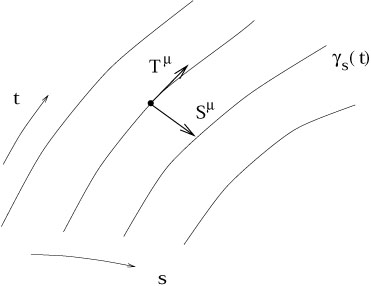
|
The idea that S![]() points from one geodesic to the next
inspires
us to define the "relative velocity of geodesics,"
points from one geodesic to the next
inspires
us to define the "relative velocity of geodesics,"
| (3.109) |
and the "relative acceleration of geodesics,"
| (3.110) |
You should take the names with a grain of salt, but these vectors are certainly well-defined.
Since S and T are basis vectors adapted to a coordinate system, their commutator vanishes:
We would like to consider the conventional case where the torsion vanishes, so from (3.70) we then have
| (3.111) |
With this in mind, let's compute the acceleration:
| (3.112) |
Let's think about this line by line. The first line is the definition
of a![]() , and the second line comes directly
from (3.111). The
third line is simply the Leibniz rule. The fourth line replaces a
double covariant derivative by the derivatives in the opposite order
plus the Riemann tensor. In the fifth line we use Leibniz again (in
the opposite order from usual), and then we cancel two identical terms
and notice that the term involving
T
, and the second line comes directly
from (3.111). The
third line is simply the Leibniz rule. The fourth line replaces a
double covariant derivative by the derivatives in the opposite order
plus the Riemann tensor. In the fifth line we use Leibniz again (in
the opposite order from usual), and then we cancel two identical terms
and notice that the term involving
T![]()
![]() T
T![]() vanishes
because T
vanishes
because T![]() is the tangent vector to a
geodesic. The result,
is the tangent vector to a
geodesic. The result,
| (3.113) |
is known as the geodesic deviation equation. It expresses something that we might have expected: the relative acceleration between two neighboring geodesics is proportional to the curvature.
Physically, of course, the acceleration of neighboring geodesics is interpreted as a manifestation of gravitational tidal forces. This reminds us that we are very close to doing physics by now.
There is one last piece of formalism which it would be nice to cover before we move on to gravitation proper. What we will do is to consider once again (although much more concisely) the formalism of connections and curvature, but this time we will use sets of basis vectors in the tangent space which are not derived from any coordinate system. It will turn out that this slight change in emphasis reveals a different point of view on the connection and curvature, one in which the relationship to gauge theories in particle physics is much more transparent. In fact the concepts to be introduced are very straightforward, but the subject is a notational nightmare, so it looks more difficult than it really is.
Up until now we have been taking advantage of the fact that a natural
basis for the tangent space Tp at a point p is
given by the
partial derivatives with respect to the coordinates at that point,
![]() =
= ![]() . Similarly, a
basis for the cotangent space T*p is given
by the gradients of the coordinate functions,
. Similarly, a
basis for the cotangent space T*p is given
by the gradients of the coordinate functions,
![]() = dx
= dx![]() . There is nothing to
stop us, however, from setting up any bases we like. Let us therefore
imagine that at each point in the manifold we introduce a set of
basis vectors
. There is nothing to
stop us, however, from setting up any bases we like. Let us therefore
imagine that at each point in the manifold we introduce a set of
basis vectors
![]() (indexed by a Latin letter rather than Greek, to
remind us that they are not related to any coordinate system). We will
choose these basis vectors to be "orthonormal", in a sense which is
appropriate to the signature of the manifold we are working on. That is,
if the canonical form of the metric is written
(indexed by a Latin letter rather than Greek, to
remind us that they are not related to any coordinate system). We will
choose these basis vectors to be "orthonormal", in a sense which is
appropriate to the signature of the manifold we are working on. That is,
if the canonical form of the metric is written ![]() , we demand
that the inner product of our basis vectors be
, we demand
that the inner product of our basis vectors be
| (3.114) |
where g( , ) is the usual metric tensor. Thus, in a Lorentzian
spacetime ![]() represents the Minkowski metric, while in a
space with positive-definite metric it would represent the Euclidean
metric. The set of vectors comprising an orthonormal basis
is sometimes known as a tetrad (from Greek tetras,
"a group of four") or vielbein (from the German
for "many legs"). In different numbers of dimensions it
occasionally becomes a vierbein (four), dreibein (three),
zweibein (two), and so on. (Just as we cannot in general find
coordinate charts which cover the entire manifold, we will often not
be able to find a single set of smooth basis vector fields which are
defined everywhere. As usual, we can overcome this problem by working
in different patches and making sure things are well-behaved on the
overlaps.)
represents the Minkowski metric, while in a
space with positive-definite metric it would represent the Euclidean
metric. The set of vectors comprising an orthonormal basis
is sometimes known as a tetrad (from Greek tetras,
"a group of four") or vielbein (from the German
for "many legs"). In different numbers of dimensions it
occasionally becomes a vierbein (four), dreibein (three),
zweibein (two), and so on. (Just as we cannot in general find
coordinate charts which cover the entire manifold, we will often not
be able to find a single set of smooth basis vector fields which are
defined everywhere. As usual, we can overcome this problem by working
in different patches and making sure things are well-behaved on the
overlaps.)
The point of having a basis is that any vector can be expressed as a
linear combination of basis vectors. Specifically, we can express our
old basis vectors
![]() =
= ![]() in terms of the new ones:
in terms of the new ones:

| (3.115) |
The components ea![]() form an n × n
invertible matrix. (In
accord with our usual practice of blurring the distinction between
objects and their components, we will refer to the
ea
form an n × n
invertible matrix. (In
accord with our usual practice of blurring the distinction between
objects and their components, we will refer to the
ea![]() as
the tetrad or vielbein, and often in the plural as "vielbeins.")
We denote their inverse by switching indices
to obtain e
as
the tetrad or vielbein, and often in the plural as "vielbeins.")
We denote their inverse by switching indices
to obtain e![]() a, which satisfy
a, which satisfy
| (3.116) |
These serve as the components of the vectors
![]() in the coordinate
basis:
in the coordinate
basis:

| (3.117) |
In terms of the inverse vielbeins, (3.114) becomes

| (3.118) |
or equivalently

| (3.119) |
This last equation sometimes leads people to say that the vielbeins are the "square root" of the metric.
We can similarly set up an orthonormal basis of one-forms in
T*p, which we denote
![]() . They may be chosen to be compatible
with the basis vectors, in the sense that
. They may be chosen to be compatible
with the basis vectors, in the sense that

| (3.120) |
It is an immediate consequence of this that the orthonormal one-forms
are related to their coordinate-based cousins
![]() = dx
= dx![]() by
by

| (3.121) |
and

| (3.122) |
The vielbeins ea![]() thus serve double duty as the
components of the
coordinate basis vectors in terms of the orthonormal basis vectors, and
as components of the orthonormal basis one-forms in terms of the
coordinate basis one-forms; while the inverse vielbeins serve as the
components of the orthonormal basis vectors in terms of the coordinate
basis, and as components of the coordinate basis one-forms in terms of
the orthonormal basis.
thus serve double duty as the
components of the
coordinate basis vectors in terms of the orthonormal basis vectors, and
as components of the orthonormal basis one-forms in terms of the
coordinate basis one-forms; while the inverse vielbeins serve as the
components of the orthonormal basis vectors in terms of the coordinate
basis, and as components of the coordinate basis one-forms in terms of
the orthonormal basis.
Any other vector can be expressed in terms of its components in the
orthonormal basis. If a vector V is written in the coordinate
basis as
V![]()
![]() and in the orthonormal basis as
Va
and in the orthonormal basis as
Va![]() ,
the sets of components will be related by
,
the sets of components will be related by

| (3.123) |
So the vielbeins allow us to "switch from Latin to Greek indices and back." The nice property of tensors, that there is usually only one sensible thing to do based on index placement, is of great help here. We can go on to refer to multi-index tensors in either basis, or even in terms of mixed components:

| (3.124) |
Looking back at (3.118), we see that the components of the metric tensor
in the orthonormal basis are just those of the flat metric,
![]() . (For this reason the Greek indices are
sometimes referred
to as "curved" and the Latin ones as "flat.") In fact we can
go so far as to raise and lower the Latin indices using the flat metric
and its inverse
. (For this reason the Greek indices are
sometimes referred
to as "curved" and the Latin ones as "flat.") In fact we can
go so far as to raise and lower the Latin indices using the flat metric
and its inverse ![]() . You can check for yourself that everything
works okay (e.g., that the lowering an index with the metric
commutes with changing from orthonormal to coordinate bases).
. You can check for yourself that everything
works okay (e.g., that the lowering an index with the metric
commutes with changing from orthonormal to coordinate bases).
By introducing a new set of basis vectors and one-forms, we necessitate a return to our favorite topic of transformation properties. We've been careful all along to emphasize that the tensor transformation law was only an indirect outcome of a coordinate transformation; the real issue was a change of basis. Now that we have non-coordinate bases, these bases can be changed independently of the coordinates. The only restriction is that the orthonormality property (3.114) be preserved. But we know what kind of transformations preserve the flat metric - in a Euclidean signature metric they are orthogonal transformations, while in a Lorentzian signature metric they are Lorentz transformations. We therefore consider changes of basis of the form
| (3.125) |
where the matrices
![]() a(x) represent
position-dependent
transformations which (at each point) leave the canonical form of the
metric unaltered:
a(x) represent
position-dependent
transformations which (at each point) leave the canonical form of the
metric unaltered:
| (3.126) |
In fact these matrices correspond to what in flat space we called
the inverse Lorentz transformations (which operate on basis vectors);
as before we also have ordinary Lorentz transformations
![]() a,
which transform the basis one-forms. As far as components are concerned,
as before we transform upper indices with
a,
which transform the basis one-forms. As far as components are concerned,
as before we transform upper indices with
![]() a and lower
indices with
a and lower
indices with
![]() a.
a.
So we now have the freedom to perform a Lorentz transformation (or an ordinary Euclidean rotation, depending on the signature) at every point in space. These transformations are therefore called local Lorentz transformations, or LLT's. We still have our usual freedom to make changes in coordinates, which are called general coordinate transformations, or GCT's. Both can happen at the same time, resulting in a mixed tensor transformation law:
| (3.127) |
Translating what we know about tensors into non-coordinate bases is
for the most part merely a matter of sticking vielbeins in the right
places. The crucial exception comes when we begin to differentiate
things. In our ordinary formalism, the covariant derivative of
a tensor is given by its partial derivative plus correction terms, one
for each index, involving the tensor and the connection coefficients.
The same procedure will continue to be true for the non-coordinate
basis, but we replace the ordinary connection coefficients
![]() by the spin connection,
denoted
by the spin connection,
denoted
![]() ab. Each Latin index gets
a factor of the spin connection in the usual way:
ab. Each Latin index gets
a factor of the spin connection in the usual way:

| (3.128) |
(The name "spin connection" comes from the fact that this can be used to take covariant derivatives of spinors, which is actually impossible using the conventional connection coefficients.) In the presence of mixed Latin and Greek indices we get terms of both kinds.
The usual demand that a tensor be independent of the way it is
written allows us to derive a relationship between the spin connection,
the vielbeins, and the
![]() 's.
Consider the covariant derivative of a vector X,
first in a purely coordinate basis:
's.
Consider the covariant derivative of a vector X,
first in a purely coordinate basis:
| (3.129) |
Now find the same object in a mixed basis, and convert into the coordinate basis:
| (3.130) |
Comparison with (3.129) reveals
| (3.131) |
or equivalently
| (3.132) |
A bit of manipulation allows us to write this relation as the vanishing of the covariant derivative of the vielbein,

| (3.133) |
which is sometimes known as the "tetrad postulate." Note that this is always true; we did not need to assume anything about the connection in order to derive it. Specifically, we did not need to assume that the connection was metric compatible or torsion free.
Since the connection may be thought of as something we need to fix up the transformation law of the covariant derivative, it should come as no surprise that the spin connection does not itself obey the tensor transformation law. Actually, under GCT's the one lower Greek index does transform in the right way, as a one-form. But under LLT's the spin connection transforms inhomogeneously, as
| (3.134) |
You are encouraged to check for yourself that this results in the proper transformation of the covariant derivative.
So far we have done nothing but empty formalism, translating things
we already knew into a new notation. But the work we are doing does
buy us two things. The first, which we already alluded to, is the
ability to describe spinor fields on spacetime and take their
covariant derivatives; we won't explore this further right now.
The second is a change in viewpoint, in which we can think of
various tensors as tensor-valued differential forms. For
example, an object like
X![]() a, which we think of as a (1,
1) tensor written with mixed
indices, can also be thought of as a "vector-valued one-form."
It has one lower Greek index, so we think of it as a one-form, but
for each value of the lower index it is a vector. Similarly a
tensor
A
a, which we think of as a (1,
1) tensor written with mixed
indices, can also be thought of as a "vector-valued one-form."
It has one lower Greek index, so we think of it as a one-form, but
for each value of the lower index it is a vector. Similarly a
tensor
A![]()
![]() ab, antisymmetric
in
ab, antisymmetric
in ![]() and
and ![]() ,
can be thought of as a "(1, 1)-tensor-valued two-form." Thus, any
tensor with some number of antisymmetric lower Greek indices and some
number of Latin indices can be thought of as a differential form, but
taking values in the tensor bundle. (Ordinary differential forms are
simply scalar-valued forms.) The usefulness of this
viewpoint comes when we consider exterior derivatives. If we want
to think of X
,
can be thought of as a "(1, 1)-tensor-valued two-form." Thus, any
tensor with some number of antisymmetric lower Greek indices and some
number of Latin indices can be thought of as a differential form, but
taking values in the tensor bundle. (Ordinary differential forms are
simply scalar-valued forms.) The usefulness of this
viewpoint comes when we consider exterior derivatives. If we want
to think of X![]() a as a vector-valued
one-form, we are tempted to take its exterior derivative:
a as a vector-valued
one-form, we are tempted to take its exterior derivative:
| (3.135) |
It is easy to check that this object transforms like a two-form (that is, according to the transformation law for (0, 2) tensors) under GCT's, but not as a vector under LLT's (the Lorentz transformations depend on position, which introduces an inhomogeneous term into the transformation law). But we can fix this by judicious use of the spin connection, which can be thought of as a one-form. (Not a tensor-valued one-form, due to the nontensorial transformation law (3.134).) Thus, the object

| (3.136) |
as you can verify at home, transforms as a proper tensor.
An immediate application of this formalism is to the expressions
for the torsion and curvature, the two tensors which characterize
any given connection. The torsion, with two antisymmetric lower
indices, can be thought of as a vector-valued two-form
T![]()
![]() a.
The curvature, which is always antisymmetric in its last two
indices, is a (1, 1)-tensor-valued two-form,
Rab
a.
The curvature, which is always antisymmetric in its last two
indices, is a (1, 1)-tensor-valued two-form,
Rab![]()
![]() .
Using our freedom to suppress indices on differential forms, we
can write the defining relations for these two tensors as
.
Using our freedom to suppress indices on differential forms, we
can write the defining relations for these two tensors as
| (3.137) |
and
| (3.138) |
These are known as the Maurer-Cartan structure equations. They are equivalent to the usual definitions; let's go through the exercise of showing this for the torsion, and you can check the curvature for yourself. We have
| (3.139) |
which is just the original definition we gave. Here we have used
(3.131), the expression for the
![]() 's in terms
of the vielbeins and spin connection. We can also express identities
obeyed by these tensors as
's in terms
of the vielbeins and spin connection. We can also express identities
obeyed by these tensors as
| (3.140) |
and

| (3.141) |
The first of these is the generalization of
R![]() [
[![]()
![]()
![]() ] = 0,
while the second is the Bianchi identity
] = 0,
while the second is the Bianchi identity
![]() R
R![]()
![]() |
|![]()
![]() ] = 0. (Sometimes both equations are called
Bianchi identities.)
] = 0. (Sometimes both equations are called
Bianchi identities.)
The form of these expressions leads to an almost irresistible temptation to define a "covariant-exterior derivative", which acts on a tensor-valued form by taking the ordinary exterior derivative and then adding appropriate terms with the spin connection, one for each Latin index. Although we won't do that here, it is okay to give in to this temptation, and in fact the right hand side of (3.137) and the left hand sides of (3.140) and (3.141) can be thought of as just such covariant-exterior derivatives. But be careful, since (3.138) cannot; you can't take any sort of covariant derivative of the spin connection, since it's not a tensor.
So far our equations have been true for general connections; let's
see what we get for the Christoffel connection. The torsion-free
requirement is just that (3.137) vanish; this does not lead immediately
to any simple statement about the coefficients of the spin connection.
Metric compatibility is expressed as the vanishing of the covariant
derivative of the metric:
![]() g = 0. We can see what this leads
to when we express the metric in the orthonormal basis, where its
components are simply
g = 0. We can see what this leads
to when we express the metric in the orthonormal basis, where its
components are simply ![]() :
:
| |
| (3.142) |
Then setting this equal to zero implies

| (3.143) |
Thus, metric compatibility is equivalent to the antisymmetry of the spin connection in its Latin indices. (As before, such a statement is only sensible if both indices are either upstairs or downstairs.) These two conditions together allow us to express the spin connection in terms of the vielbeins. There is an explicit formula which expresses this solution, but in practice it is easier to simply solve the torsion-free condition
| (3.144) |
using the asymmetry of the spin connection, to find the individual components.
We now have the means to compare the formalism of connections and curvature in Riemannian geometry to that of gauge theories in particle physics. (This is an aside, which is hopefully comprehensible to everybody, but not an essential ingredient of the course.) In both situations, the fields of interest live in vector spaces which are assigned to each point in spacetime. In Riemannian geometry the vector spaces include the tangent space, the cotangent space, and the higher tensor spaces constructed from these. In gauge theories, on the other hand, we are concerned with "internal" vector spaces. The distinction is that the tangent space and its relatives are intimately associated with the manifold itself, and were naturally defined once the manifold was set up; an internal vector space can be of any dimension we like, and has to be defined as an independent addition to the manifold. In math lingo, the union of the base manifold with the internal vector spaces (defined at each point) is a fiber bundle, and each copy of the vector space is called the "fiber" (in perfect accord with our definition of the tangent bundle).
Besides the base manifold (for us, spacetime) and the fibers, the other
important ingredient in the definition of a fiber bundle is the
"structure group," a Lie group which acts on the fibers to describe
how they are sewn together on overlapping coordinate patches. Without
going into details, the structure group for the tangent bundle in a
four-dimensional spacetime is generally GL
(4,![]() ), the group of
real invertible 4 × 4 matrices; if we have a Lorentzian metric,
this may be reduced to the Lorentz group SO(3, 1). Now imagine that
we introduce an internal three-dimensional vector space, and sew the
fibers together with ordinary rotations; the structure group of
this new bundle is then SO(3). A field that lives in this
bundle might be denoted
), the group of
real invertible 4 × 4 matrices; if we have a Lorentzian metric,
this may be reduced to the Lorentz group SO(3, 1). Now imagine that
we introduce an internal three-dimensional vector space, and sew the
fibers together with ordinary rotations; the structure group of
this new bundle is then SO(3). A field that lives in this
bundle might be denoted
![]() (x
(x![]() ), where A runs from one
to three; it is a three-vector (an internal one, unrelated to
spacetime) for each point on the manifold. We have freedom to choose
the basis in the fibers in any way we wish; this means that "physical
quantities" should be left invariant under local SO(3) transformations
such as
), where A runs from one
to three; it is a three-vector (an internal one, unrelated to
spacetime) for each point on the manifold. We have freedom to choose
the basis in the fibers in any way we wish; this means that "physical
quantities" should be left invariant under local SO(3) transformations
such as
| (3.145) |
where
OA'A(x![]() ) is a matrix in SO(3) which depends on
spacetime. Such transformations are known as gauge transformations,
and theories invariant under them are called "gauge theories."
) is a matrix in SO(3) which depends on
spacetime. Such transformations are known as gauge transformations,
and theories invariant under them are called "gauge theories."
For the most part it is not hard to arrange things such that physical
quantities are invariant under gauge transformations. The one
difficulty arises when we consider partial derivatives,
![]()
![]() .
Because the matrix
OA'A(x
.
Because the matrix
OA'A(x![]() ) depends on spacetime, it will
contribute an unwanted term to the transformation of the partial derivative.
By now you should be able to guess the solution: introduce a connection
to correct for the inhomogeneous term in the transformation law. We
therefore define a connection on the fiber bundle to be an object
A
) depends on spacetime, it will
contribute an unwanted term to the transformation of the partial derivative.
By now you should be able to guess the solution: introduce a connection
to correct for the inhomogeneous term in the transformation law. We
therefore define a connection on the fiber bundle to be an object
A![]() AB, with two
"group indices" and one spacetime index.
Under GCT's it transforms as a one-form, while under gauge transformations
it transforms as
AB, with two
"group indices" and one spacetime index.
Under GCT's it transforms as a one-form, while under gauge transformations
it transforms as

| (3.146) |
(Beware: our conventions are so drastically different from those in the particle physics literature that I won't even try to get them straight.) With this transformation law, the "gauge covariant derivative"
| (3.147) |
transforms "tensorially" under gauge transformations, as you are welcome to check. (In ordinary electromagnetism the connection is just the conventional vector potential. No indices are necessary, because the structure group U(1) is one-dimensional.)
It is clear that this notion of a connection on an internal fiber bundle is very closely related to the connection on the tangent bundle, especially in the orthonormal-frame picture we have been discussing. The transformation law (3.146), for example, is exactly the same as the transformation law (3.134) for the spin connection. We can also define a curvature or "field strength" tensor which is a two-form,
| (3.148) |
in exact correspondence with (3.138). We can parallel transport things along paths, and there is a construction analogous to the parallel propagator; the trace of the matrix obtained by parallel transporting a vector around a closed curve is called a "Wilson loop."
We could go on in the development of the relationship between the tangent bundle and internal vector bundles, but time is short and we have other fish to fry. Let us instead finish by emphasizing the important difference between the two constructions. The difference stems from the fact that the tangent bundle is closely related to the base manifold, while other fiber bundles are tacked on after the fact. It makes sense to say that a vector in the tangent space at p "points along a path" through p; but this makes no sense for an internal vector bundle. There is therefore no analogue of the coordinate basis for an internal space -- partial derivatives along curves have nothing to do with internal vectors. It follows in turn that there is nothing like the vielbeins, which relate orthonormal bases to coordinate bases. The torsion tensor, in particular, is only defined for a connection on the tangent bundle, not for any gauge theory connections; it can be thought of as the covariant exterior derivative of the vielbein, and no such construction is available on an internal bundle. You should appreciate the relationship between the different uses of the notion of a connection, without getting carried away.