


With an understanding of how the laws of physics adapt to curved spacetime, it is undeniably tempting to start in on applications. However, a few extra mathematical techniques will simplify our task a great deal, so we will pause briefly to explore the geometry of manifolds some more.
When we discussed manifolds in section 2, we introduced maps
between two different manifolds and how maps could be composed. We
now turn to the use of such maps in carrying along tensor fields
from one manifold to another. We therefore consider two manifolds
M and N, possibly of different dimension, with coordinate
systems x![]() and y
and y![]() , respectively. We imagine that we have a
map
, respectively. We imagine that we have a
map
![]() : M
: M ![]() N and a function
f : N
N and a function
f : N ![]()
![]() .
.

|
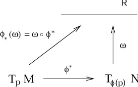
It is obvious that we can compose ![]() with f to
construct a map
(fo
with f to
construct a map
(fo![]() ) : M
) : M ![]()
![]() , which is simply
a function on M. Such a construction is sufficiently useful that
it gets its own name; we define the pullback of f by
, which is simply
a function on M. Such a construction is sufficiently useful that
it gets its own name; we define the pullback of f by ![]() ,
denoted
,
denoted ![]() f, by
f, by

| (5.1) |
The name makes sense, since we think of ![]() as "pulling back"
the function f from N to M.
as "pulling back"
the function f from N to M.
We can pull functions back, but we cannot push them forward. If
we have a function
g : M ![]()
![]() , there is no way we can compose
g with
, there is no way we can compose
g with ![]() to create a function on N; the arrows don't fit
together correctly. But recall that a vector can be thought of
as a derivative operator that maps smooth functions to real numbers.
This allows us to define the pushforward of a vector; if
V(p) is
a vector at a point p on M, we define the pushforward
vector
to create a function on N; the arrows don't fit
together correctly. But recall that a vector can be thought of
as a derivative operator that maps smooth functions to real numbers.
This allows us to define the pushforward of a vector; if
V(p) is
a vector at a point p on M, we define the pushforward
vector ![]() V
at the point
V
at the point ![]() (p) on N by giving its action on functions
on N:
(p) on N by giving its action on functions
on N:
| (5.2) |
So to push forward a vector field we say "the action of
![]() V on any function is simply the action of
V on the pullback of that function."
V on any function is simply the action of
V on the pullback of that function."
This is a little abstract, and it would be nice to have a more concrete
description. We know that a basis for vectors on M is given by
the set of partial derivatives
![]() =
= ![]() ,
and a basis on N is given by the set of partial derivatives
,
and a basis on N is given by the set of partial derivatives
![]() =
= ![]() . Therefore we would like
to relate the components of
V = V
. Therefore we would like
to relate the components of
V = V![]()
![]() to those of
(
to those of
(![]() V) = (
V) = (![]() V)
V)![]()
![]() . We can find the sought-after relation by
applying the
pushed-forward vector to a test function and using the chain
rule (2.3):
. We can find the sought-after relation by
applying the
pushed-forward vector to a test function and using the chain
rule (2.3):
| (5.3) |
This simple formula makes it irresistible to think of the pushforward
operation ![]() as a matrix operator,
(
as a matrix operator,
(![]() V)
V)![]() = (
= (![]() )
)![]()
![]() V
V![]() , with the matrix being given by
, with the matrix being given by

| (5.4) |
The behavior of a vector under a pushforward thus bears an
unmistakable resemblance to the vector transformation law under
change of coordinates. In fact it is a generalization, since when
M and N are the same manifold the constructions are (as we
shall discuss) identical; but
don't be fooled, since in general ![]() and
and ![]() have different
allowed values, and there is no reason for the matrix
have different
allowed values, and there is no reason for the matrix
![]() y
y![]() /
/![]() x
x![]() to be invertible.
to be invertible.
It is a rewarding exercise to convince yourself that, although you can
push vectors forward from M to N (given a map
![]() : M
: M ![]() N), you cannot in general pull them back -
just keep trying
to invent an appropriate construction until the futility of the attempt
becomes clear. Since one-forms are dual to vectors, you should
not be surprised to hear that one-forms can be pulled back (but not
in general pushed forward). To do this, remember that one-forms are linear
maps from vectors to the real numbers. The pullback
N), you cannot in general pull them back -
just keep trying
to invent an appropriate construction until the futility of the attempt
becomes clear. Since one-forms are dual to vectors, you should
not be surprised to hear that one-forms can be pulled back (but not
in general pushed forward). To do this, remember that one-forms are linear
maps from vectors to the real numbers. The pullback
![]()
![]() of a
one-form
of a
one-form ![]() on N can therefore be defined by its action on
a vector V on M, by equating it with the action of
on N can therefore be defined by its action on
a vector V on M, by equating it with the action of ![]() itself on the pushforward of V:
itself on the pushforward of V:
| (5.5) |
Once again, there is a simple matrix description of the pullback
operator on forms,
(![]()
![]() )
)![]() = (
= (![]() )
)![]()
![]()
![]() , which we can derive using the chain
rule. It is given by
, which we can derive using the chain
rule. It is given by

| (5.6) |
That is, it is the same matrix as the pushforward (5.4), but of course a different index is contracted when the matrix acts to pull back one-forms.
There is a way of thinking about why pullbacks and pushforwards work
on some objects but not others, which may or may not be helpful.
If we denote the set of smooth functions on M by
![]() (M),
then a vector V(p) at a point p on M
(i.e., an element of
the tangent space TpM) can be thought of as an
operator from
(M),
then a vector V(p) at a point p on M
(i.e., an element of
the tangent space TpM) can be thought of as an
operator from
![]() (M) to
(M) to ![]() . But we already know that the pullback operator
on functions maps
. But we already know that the pullback operator
on functions maps
![]() (N) to
(N) to
![]() (M) (just as
(M) (just as ![]() itself maps M to N, but in the opposite direction). Therefore
we can define the pushforward
itself maps M to N, but in the opposite direction). Therefore
we can define the pushforward ![]() acting on vectors simply by
composing maps, as we first defined the pullback of functions:
acting on vectors simply by
composing maps, as we first defined the pullback of functions:

|
Similarly, if TqN is the tangent space at a
point q on N,
then a one-form ![]() at q
(i.e., an element of the cotangent space
Tq*N) can be thought of
as an operator from TqN to
at q
(i.e., an element of the cotangent space
Tq*N) can be thought of
as an operator from TqN to ![]() . Since the pushforward
. Since the pushforward
![]() maps TpM to
T
maps TpM to
T![]() (p)N, the pullback
(p)N, the pullback ![]() of a one-form can also be thought of as mere composition of maps:
of a one-form can also be thought of as mere composition of maps:
|
If this is not helpful, don't worry about it. But do keep straight what exists and what doesn't; the actual concepts are simple, it's just remembering which map goes what way that leads to confusion.
You will recall further that a (0, l ) tensor - one with l
lower
indices and no upper ones - is a linear map from the direct product
of l vectors to ![]() . We can therefore pull back not only one-forms,
but tensors with an arbitrary number of lower indices. The definition
is simply the action of the original tensor on the pushed-forward
vectors:
. We can therefore pull back not only one-forms,
but tensors with an arbitrary number of lower indices. The definition
is simply the action of the original tensor on the pushed-forward
vectors:

| (5.7) |
where
T![]() ...
... ![]() is a (0, l ) tensor on
N. We can
similarly push forward any (k, 0) tensor
S
is a (0, l ) tensor on
N. We can
similarly push forward any (k, 0) tensor
S![]() ...
... ![]() by acting it on pulled-back one-forms:
by acting it on pulled-back one-forms:

| (5.8) |
Fortunately, the matrix representations of the pushforward (5.4) and pullback (5.6) extend to the higher-rank tensors simply by assigning one matrix to each index; thus, for the pullback of a (0, l ) tensor, we have
| (5.9) |
while for the pushforward of a (k, 0) tensor we have
| (5.10) |
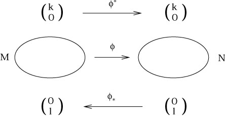
Our complete picture is therefore:
|
Note that tensors with both upper and lower indices can generally be neither pushed forward nor pulled back.
This machinery becomes somewhat less imposing once we see it at work
in a simple example. One common occurrence of a map between two
manifolds is when M is actually a submanifold of N; then
there is
an obvious map from M to N which just takes an element of
M to
the "same" element of N. Consider our usual example, the two-sphere
embedded in ![]() , as the locus of points a unit distance from the
origin. If we put coordinates
x
, as the locus of points a unit distance from the
origin. If we put coordinates
x![]() = (
= (![]() ,
,![]() ) on M = S2 and
y
) on M = S2 and
y![]() = (x, y, z) on
N =
= (x, y, z) on
N = ![]() , the map
, the map
![]() : M
: M ![]() N is given by
N is given by

| (5.11) |
In the past we have considered the metric
ds2 = dx2 + dy2 +
dz2
on ![]() , and said that it induces a metric
d
, and said that it induces a metric
d![]() + sin2
+ sin2![]() d
d![]() on S2, just by substituting
(5.11) into this flat metric
on
on S2, just by substituting
(5.11) into this flat metric
on ![]() . We didn't really justify such a statement at the
time, but now we can do so. (Of course it would be easier if we
worked in spherical coordinates on
. We didn't really justify such a statement at the
time, but now we can do so. (Of course it would be easier if we
worked in spherical coordinates on ![]() , but doing it the hard way
is more illustrative.) The matrix of partial derivatives is given
by
, but doing it the hard way
is more illustrative.) The matrix of partial derivatives is given
by
| (5.12) |
The metric on S2 is obtained by simply pulling back
the metric from
![]() ,
,
| (5.13) |
as you can easily check. Once again, the answer is the same as you would get by naive substitution, but now we know why.
We have been careful to emphasize that a map
![]() : M
: M ![]() N can
be used to push certain things forward and pull other things back.
The reason why it generally doesn't work both ways can be traced to the
fact that
N can
be used to push certain things forward and pull other things back.
The reason why it generally doesn't work both ways can be traced to the
fact that ![]() might not be invertible. If
might not be invertible. If ![]() is invertible
(and both
is invertible
(and both ![]() and
and ![]() are smooth, which we always implicitly
assume), then it defines a diffeomorphism between M and
N. In this
case M and N are the same abstract manifold. The beauty
of diffeomorphisms is that we can use both
are smooth, which we always implicitly
assume), then it defines a diffeomorphism between M and
N. In this
case M and N are the same abstract manifold. The beauty
of diffeomorphisms is that we can use both ![]() and
and ![]() to
move tensors from M to N; this will allow us to define the
pushforward and pullback of arbitrary tensors. Specifically, for a
(k, l ) tensor field
T
to
move tensors from M to N; this will allow us to define the
pushforward and pullback of arbitrary tensors. Specifically, for a
(k, l ) tensor field
T![]() ...
... ![]()
![]() ...
... ![]() on M, we define the pushforward by
on M, we define the pushforward by

| (5.14) |
where the
![]() 's are one-forms on N and the
V(i)'s
are vectors on N. In components this becomes
's are one-forms on N and the
V(i)'s
are vectors on N. In components this becomes
| (5.15) |
The appearance of the inverse matrix
![]() x
x![]() /
/![]() y
y![]() is legitimate because
is legitimate because ![]() is invertible. Note that we could also
define the pullback in the obvious way, but there is no need to write
separate equations because the pullback
is invertible. Note that we could also
define the pullback in the obvious way, but there is no need to write
separate equations because the pullback ![]() is the same as the
pushforward via the inverse map,
[
is the same as the
pushforward via the inverse map,
[![]() ]*.
]*.
We are now in a position to explain the relationship between
diffeomorphisms and coordinate transformations. The relationship is
that they are two different ways of doing precisely the same thing.
If you like, diffeomorphisms are "active coordinate transformations",
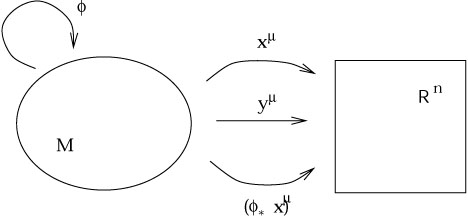
while traditional coordinate transformations are "passive." Consider
an n-dimensional manifold M with coordinate functions
x![]() : M
: M ![]()
![]() . To change coordinates we can either simply
introduce new functions
y
. To change coordinates we can either simply
introduce new functions
y![]() : M
: M ![]()
![]() ("keep the manifold
fixed, change the coordinate maps"), or we could just as well introduce
a diffeomorphism
("keep the manifold
fixed, change the coordinate maps"), or we could just as well introduce
a diffeomorphism
![]() : M
: M ![]() M, after which the coordinates would
just be the pullbacks
(
M, after which the coordinates would
just be the pullbacks
(![]() x)
x)![]() : M
: M ![]()
![]() ("move the
points on the manifold, and then evaluate the coordinates of the new
points"). In this sense, (5.15) really is the tensor transformation
law, just thought of from a different point of view.
("move the
points on the manifold, and then evaluate the coordinates of the new
points"). In this sense, (5.15) really is the tensor transformation
law, just thought of from a different point of view.
|
Since a diffeomorphism allows us to pull back and push forward arbitrary
tensors, it provides another way of comparing tensors at different
points on a manifold. Given a diffeomorphism
![]() : M
: M ![]() M and
a tensor field
T
M and
a tensor field
T![]() ...
... ![]()
![]() ...
... ![]() (x), we
can form the difference between the value of the tensor at some point
p and
(x), we
can form the difference between the value of the tensor at some point
p and
![]() [T
[T![]() ...
... ![]()
![]() ...
... ![]() (
(![]() (p))],
its value at
(p))],
its value at ![]() (p) pulled back to p.
This suggests that we could define another kind of derivative operator
on tensor fields, one which categorizes the rate of change of the
tensor as it changes under the diffeomorphism. For that, however, a
single discrete diffeomorphism is insufficient; we require a one-parameter
family of diffeomorphisms,
(p) pulled back to p.
This suggests that we could define another kind of derivative operator
on tensor fields, one which categorizes the rate of change of the
tensor as it changes under the diffeomorphism. For that, however, a
single discrete diffeomorphism is insufficient; we require a one-parameter
family of diffeomorphisms, ![]() . This family can be thought of as
a smooth map
. This family can be thought of as
a smooth map
![]() x M
x M ![]() M, such that for each
t
M, such that for each
t ![]()
![]()
![]() is a diffeomorphism and
is a diffeomorphism and
![]() o
o![]() =
= ![]() . Note
that this last condition implies that
. Note
that this last condition implies that ![]() is the identity map.
is the identity map.
One-parameter families of diffeomorphisms can be thought of as arising
from vector fields (and vice-versa). If we consider what happens to
the point p under the entire family ![]() , it is clear that it
describes a curve in M; since the same thing will be true of every
point on M, these curves fill the manifold (although there can be
degeneracies where the diffeomorphisms have fixed points). We can define
a vector field V
, it is clear that it
describes a curve in M; since the same thing will be true of every
point on M, these curves fill the manifold (although there can be
degeneracies where the diffeomorphisms have fixed points). We can define
a vector field V![]() (x) to be the set of tangent
vectors to each of
these curves at every point, evaluated at t = 0. An example on
S2
is provided by the diffeomorphism
(x) to be the set of tangent
vectors to each of
these curves at every point, evaluated at t = 0. An example on
S2
is provided by the diffeomorphism
![]() (
(![]() ,
,![]() ) = (
) = (![]() ,
,![]() + t).
+ t).

|
We can reverse the construction to define a one-parameter family of
diffeomorphisms from any vector field. Given a vector field
V![]() (x), we define the integral
curves of the vector field
to be those curves x
(x), we define the integral
curves of the vector field
to be those curves x![]() (t) which solve
(t) which solve

| (5.16) |
Note that this familiar-looking equation is now to be interpreted
in the opposite sense from our usual way - we are given the vectors,
from which we define the curves. Solutions to (5.16) are guaranteed
to exist as long as we don't do anything silly like run into the
edge of our manifold; any standard differential geometry text will
have the proof, which amounts to finding a clever coordinate system in
which the problem reduces to the fundamental theorem of ordinary
differential equations. Our diffeomorphisms ![]() represent "flow
down the integral curves," and the associated vector field is referred
to as the generator of the diffeomorphism. (Integral curves are
used all the time in elementary physics, just not given the name.
The "lines of magnetic flux" traced out by iron filings in the
presence of a magnet are simply the integral curves of the magnetic
field vector B.)
represent "flow
down the integral curves," and the associated vector field is referred
to as the generator of the diffeomorphism. (Integral curves are
used all the time in elementary physics, just not given the name.
The "lines of magnetic flux" traced out by iron filings in the
presence of a magnet are simply the integral curves of the magnetic
field vector B.)
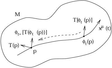
Given a vector field V![]() (x), then, we have a family of
diffeomorphisms parameterized by t, and we can ask how fast a tensor
changes as we travel down the integral curves. For each t we can
define this change as
(x), then, we have a family of
diffeomorphisms parameterized by t, and we can ask how fast a tensor
changes as we travel down the integral curves. For each t we can
define this change as

| (5.17) |
Note that both terms on the right hand side are tensors at p.
|
We then define the Lie derivative of the tensor along the vector field as
| (5.18) |
The Lie derivative is a map from (k, l ) tensor fields to (k, l ) tensor fields, which is manifestly independent of coordinates. Since the definition essentially amounts to the conventional definition of an ordinary derivative applied to the component functions of the tensor, it should be clear that it is linear,

| (5.19) |
and obeys the Leibniz rule,

| (5.20) |
where S and T are tensors and a and b are constants. The Lie derivative is in fact a more primitive notion than the covariant derivative, since it does not require specification of a connection (although it does require a vector field, of course). A moment's reflection shows that it reduces to the ordinary derivative on functions,
| (5.21) |
To discuss the action of the Lie derivative on tensors in terms of
other operations we know, it is convenient to choose a coordinate
system adapted to our problem. Specifically, we will work in
coordinates x![]() for which x1 is the
parameter along the
integral curves (and the other coordinates
are chosen any way we like). Then the vector field takes the form
V =
for which x1 is the
parameter along the
integral curves (and the other coordinates
are chosen any way we like). Then the vector field takes the form
V = ![]() /
/![]() x1; that is, it has components
V
x1; that is, it has components
V![]() = (1, 0, 0,..., 0). The magic of this
coordinate system is that a
diffeomorphism by t amounts to a coordinate transformation from
x
= (1, 0, 0,..., 0). The magic of this
coordinate system is that a
diffeomorphism by t amounts to a coordinate transformation from
x![]() to
y
to
y![]() = (x1 + t,
x2,..., xn). Thus, from (5.6) the
pullback matrix is simply
= (x1 + t,
x2,..., xn). Thus, from (5.6) the
pullback matrix is simply

| (5.22) |
and the components of the tensor pulled back from ![]() (p) to
p are simply
(p) to
p are simply

| (5.23) |
In this coordinate system, then, the Lie derivative becomes
| (5.24) |
and specifically the derivative of a vector field U![]() (x) is
(x) is
| (5.25) |
Although this expression is clearly not covariant, we know that the commutator [V, U] is a well-defined tensor, and in this coordinate system
| (5.26) |
Therefore the Lie derivative of U with respect to V has the same components in this coordinate system as the commutator of V and U; but since both are vectors, they must be equal in any coordinate system:
| (5.27) |
As an immediate consequence, we have £VS = - £WV. It is because of (5.27) that the commutator is sometimes called the "Lie bracket."
To derive the action of
£V on a one-form
![]() ,
begin by considering the action on the scalar
,
begin by considering the action on the scalar
![]() U
U![]() for an arbitrary vector field U
for an arbitrary vector field U![]() . First use the fact that
the Lie derivative with respect to a vector field reduces to the action
of the vector itself when applied to a scalar:
. First use the fact that
the Lie derivative with respect to a vector field reduces to the action
of the vector itself when applied to a scalar:
| (5.28) |
Then use the Leibniz rule on the original scalar:
| (5.29) |
Setting these expressions equal to each other and requiring that
equality hold for arbitrary U![]() , we see that
, we see that
| (5.30) |
which (like the definition of the commutator) is completely covariant, although not manifestly so.
By a similar procedure we can define the Lie derivative of an arbitrary tensor field. The answer can be written
| (5.31) |
Once again, this expression is covariant, despite appearances. It would undoubtedly be comforting, however, to have an equivalent expression that looked manifestly tensorial. In fact it turns out that we can write
| (5.32) |
where
![]() represents any symmetric (torsion-free)
covariant derivative (including, of course, one derived from a
metric). You can check that all of the terms which would involve
connection coefficients if we were to expand (5.32) would cancel,
leaving only (5.31). Both versions of the formula for a Lie derivative
are useful at different times. A particularly useful formula is for
the Lie derivative of the metric:
represents any symmetric (torsion-free)
covariant derivative (including, of course, one derived from a
metric). You can check that all of the terms which would involve
connection coefficients if we were to expand (5.32) would cancel,
leaving only (5.31). Both versions of the formula for a Lie derivative
are useful at different times. A particularly useful formula is for
the Lie derivative of the metric:
| (5.33) |
where
![]() is the covariant derivative derived from
g
is the covariant derivative derived from
g![]()
![]() .
.
Let's put some of these ideas into the context of general relativity.
You will often hear it proclaimed that GR is a "diffeomorphism
invariant" theory. What this means is that, if the universe is
represented by a manifold M with metric
g![]()
![]() and matter fields
and matter fields
![]() , and
, and
![]() : M
: M ![]() M is a diffeomorphism, then the sets
(M, g
M is a diffeomorphism, then the sets
(M, g![]()
![]() ,
,![]() ) and
(M,
) and
(M,![]() g
g![]()
![]() ,
,![]()
![]() ) represent the same
physical situation. Since diffeomorphisms are just active coordinate
transformations, this is a highbrow way of saying that the theory is
coordinate invariant. Although such a statement is true, it is a
source of great misunderstanding, for the simple fact that it conveys
very little information. Any semi-respectable theory of physics is
coordinate invariant, including those based on special relativity or
Newtonian mechanics; GR is not unique in this regard. When people say
that GR is diffeomorphism invariant, more likely than not they have one
of two (closely related) concepts in mind: the theory is free of "prior
geometry", and there is no preferred coordinate system for spacetime.
The first of these stems from the fact that the metric is a
dynamical variable, and along with it the connection and volume
element and so forth. Nothing is given to us ahead of time, unlike in
classical mechanics or SR. As a consequence, there is no way to
simplify life by sticking to a specific coordinate system adapted to
some absolute elements of the geometry. This state of affairs forces
us to be very careful; it is possible that two purportedly distinct
configurations (of matter and metric) in GR are actually "the same",
related by a diffeomorphism. In a path integral approach to quantum
gravity, where we would like to sum over all possible configurations,
special care must be taken not to overcount by allowing physically
indistinguishable configurations to contribute more than once. In
SR or Newtonian mechanics, meanwhile, the existence of a preferred
set of coordinates saves us from such ambiguities. The fact that GR
has no preferred coordinate system is often garbled into the
statement that it is coordinate invariant (or "generally covariant");
both things are true, but one has more content than the other.
) represent the same
physical situation. Since diffeomorphisms are just active coordinate
transformations, this is a highbrow way of saying that the theory is
coordinate invariant. Although such a statement is true, it is a
source of great misunderstanding, for the simple fact that it conveys
very little information. Any semi-respectable theory of physics is
coordinate invariant, including those based on special relativity or
Newtonian mechanics; GR is not unique in this regard. When people say
that GR is diffeomorphism invariant, more likely than not they have one
of two (closely related) concepts in mind: the theory is free of "prior
geometry", and there is no preferred coordinate system for spacetime.
The first of these stems from the fact that the metric is a
dynamical variable, and along with it the connection and volume
element and so forth. Nothing is given to us ahead of time, unlike in
classical mechanics or SR. As a consequence, there is no way to
simplify life by sticking to a specific coordinate system adapted to
some absolute elements of the geometry. This state of affairs forces
us to be very careful; it is possible that two purportedly distinct
configurations (of matter and metric) in GR are actually "the same",
related by a diffeomorphism. In a path integral approach to quantum
gravity, where we would like to sum over all possible configurations,
special care must be taken not to overcount by allowing physically
indistinguishable configurations to contribute more than once. In
SR or Newtonian mechanics, meanwhile, the existence of a preferred
set of coordinates saves us from such ambiguities. The fact that GR
has no preferred coordinate system is often garbled into the
statement that it is coordinate invariant (or "generally covariant");
both things are true, but one has more content than the other.
On the other hand, the fact of diffeomorphism invariance can be put
to good use. Recall that the complete action for gravity coupled to
a set of matter fields ![]() is given by a sum of the Hilbert action
for GR plus the matter action,
is given by a sum of the Hilbert action
for GR plus the matter action,
| (5.34) |
The Hilbert action SH is diffeomorphism invariant when considered in isolation, so the matter action SM must also be if the action as a whole is to be invariant. We can write the variation in SM under a diffeomorphism as
| (5.35) |
We are not considering arbitrary variations of the fields, only those
which result from a diffeomorphism. Nevertheless, the matter equations
of motion tell us that the variation of SM with
respect to ![]() will vanish for any variation (since the gravitational part of the action
doesn't involve the matter fields). Hence, for a diffeomorphism
invariant theory the first term on the right hand side of (5.35) must
vanish. If the diffeomorphism in generated by a vector field
V
will vanish for any variation (since the gravitational part of the action
doesn't involve the matter fields). Hence, for a diffeomorphism
invariant theory the first term on the right hand side of (5.35) must
vanish. If the diffeomorphism in generated by a vector field
V![]() (x),
the infinitesimal change in the metric is simply given by its Lie
derivative along V
(x),
the infinitesimal change in the metric is simply given by its Lie
derivative along V![]() ; by (5.33) we have
; by (5.33) we have
| (5.36) |
Setting
![]() SM = 0 then implies
SM = 0 then implies
| (5.37) |
where we are able to drop the symmetrization of
![]() V
V![]() )
since
)
since
![]() SM/
SM/![]() g
g![]()
![]() is already symmetric. Demanding that
(5.37) hold for diffeomorphisms generated by arbitrary vector fields
V
is already symmetric. Demanding that
(5.37) hold for diffeomorphisms generated by arbitrary vector fields
V![]() , and using the definition (4.70) of the
energy-momentum tensor,
we obtain precisely the law of energy-momentum conservation,
, and using the definition (4.70) of the
energy-momentum tensor,
we obtain precisely the law of energy-momentum conservation,

| (5.38) |
This is why we claimed earlier that the conservation of
T![]()
![]() was
more than simply a consequence of the Principle of Equivalence; it is
much more secure than that, resting only on the diffeomorphism
invariance of the theory.
was
more than simply a consequence of the Principle of Equivalence; it is
much more secure than that, resting only on the diffeomorphism
invariance of the theory.
There is one more use to which we will put the machinery we have
set up in this section: symmetries of tensors. We say that a
diffeomorphism ![]() is a symmetry of some tensor
T if the tensor is invariant after being pulled back under
is a symmetry of some tensor
T if the tensor is invariant after being pulled back under ![]() :
:

| (5.39) |
Although symmetries may be discrete, it is more common to have a
one-parameter family of symmetries ![]() . If the family is
generated by a vector field V
. If the family is
generated by a vector field V![]() (x), then (5.39) amounts to
(x), then (5.39) amounts to

| (5.40) |
By (5.25), one implication of a symmetry is that, if T is symmetric under some one-parameter family of diffeomorphisms, we can always find a coordinate system in which the components of T are all independent of one of the coordinates (the integral curve coordinate of the vector field). The converse is also true; if all of the components are independent of one of the coordinates, then the partial derivative vector field associated with that coordinate generates a symmetry of the tensor.
The most important symmetries are those of the metric, for which
![]() g
g![]()
![]() = g
= g![]()
![]() . A diffeomorphism of this type is called an
isometry. If a one-parameter family of isometries is
generated by a vector field V
. A diffeomorphism of this type is called an
isometry. If a one-parameter family of isometries is
generated by a vector field V![]() (x), then V
(x), then V![]() is known as
a Killing vector field. The condition that V
is known as
a Killing vector field. The condition that V![]() be a Killing
vector is thus
be a Killing
vector is thus

| (5.41) |
or from (5.33),

| (5.42) |
This last version is Killing's equation. If a spacetime has a Killing vector, then we know we can find a coordinate system in which the metric is independent of one of the coordinates.
By far the most useful fact about Killing vectors is that Killing
vectors imply conserved quantities associated with the motion of
free particles. If
x![]() (
(![]() ) is a geodesic with tangent
vector
U
) is a geodesic with tangent
vector
U![]() = dx
= dx![]() /d
/d![]() , and V
, and V![]() is a Killing vector, then
is a Killing vector, then
| (5.43) |
where the first term vanishes from Killing's equation and the second
from the fact that
x![]() (
(![]() ) is a geodesic. Thus, the
quantity
V
) is a geodesic. Thus, the
quantity
V![]() U
U![]() is conserved along the particle's
worldline.
This can be understood physically: by definition the metric is
unchanging along the direction of the Killing vector. Loosely speaking,
therefore, a free particle will not feel any "forces"
in this direction, and the component of its momentum in that
direction will consequently be conserved.
is conserved along the particle's
worldline.
This can be understood physically: by definition the metric is
unchanging along the direction of the Killing vector. Loosely speaking,
therefore, a free particle will not feel any "forces"
in this direction, and the component of its momentum in that
direction will consequently be conserved.
Long ago we referred to the concept of a space with maximal symmetry,
without offering a rigorous definition. The rigorous
definition is that a maximally symmetric space is one which
possesses the largest possible number of Killing vectors, which on
an n-dimensional manifold is n(n + 1)/2. We will
not prove
this statement, but it is easy to understand at an informal level.
Consider the Euclidean space ![]() , where the isometries are well
known to us: translations and rotations. In general there will
be n translations, one for each direction we can move. There will
also be n(n - 1)/2 rotations; for each of n
dimensions there are
n - 1 directions in which we can rotate it, but we must divide by
two to prevent overcounting (rotating x into y and
rotating y
into x are two versions of the same thing). We therefore have
, where the isometries are well
known to us: translations and rotations. In general there will
be n translations, one for each direction we can move. There will
also be n(n - 1)/2 rotations; for each of n
dimensions there are
n - 1 directions in which we can rotate it, but we must divide by
two to prevent overcounting (rotating x into y and
rotating y
into x are two versions of the same thing). We therefore have

| (5.44) |
independent Killing vectors. The same kind of counting argument applies to maximally symmetric spaces with curvature (such as spheres) or a non-Euclidean signature (such as Minkowski space), although the details are marginally different.
Although it may or may not be simple to actually solve Killing's
equation in any given spacetime, it is frequently possible to
write down some Killing vectors by inspection. (Of course a "generic"
metric has no Killing vectors at all, but to keep things simple we
often deal with metrics with high degrees of symmetry.) For example
in ![]() with metric
ds2 = dx2 + dy2,
independence of the
metric components with respect to x and y immediately
yields two Killing vectors:
with metric
ds2 = dx2 + dy2,
independence of the
metric components with respect to x and y immediately
yields two Killing vectors:

| (5.45) |
These clearly
represent the two translations. The one rotation would correspond to
the vector
R = ![]() /
/![]()
![]() if we were in polar coordinates;
in Cartesian coordinates this becomes
if we were in polar coordinates;
in Cartesian coordinates this becomes

| (5.46) |
You can check for yourself that this actually does solve Killing's equation.
Note that in n ![]() 2 dimensions, there can be more Killing vectors
than dimensions. This is because a set of Killing vector fields can
be linearly independent, even though at any one point on the manifold
the vectors at that point are linearly dependent. It is trivial to
show (so you should do it yourself) that a linear combination
of Killing vectors with constant coefficients is still a Killing
vector (in which case the linear combination does not count as an
independent Killing vector),
but this is not necessarily true with coefficients which
vary over the manifold. You will also show that the commutator of two
Killing vector fields is a Killing vector field; this is very useful
to know, but it may be the case that the commutator gives you a vector
field which is not linearly independent (or it may simply vanish).
The problem of finding all of the Killing vectors of a metric is therefore
somewhat tricky, as it is sometimes not clear when to stop looking.
2 dimensions, there can be more Killing vectors
than dimensions. This is because a set of Killing vector fields can
be linearly independent, even though at any one point on the manifold
the vectors at that point are linearly dependent. It is trivial to
show (so you should do it yourself) that a linear combination
of Killing vectors with constant coefficients is still a Killing
vector (in which case the linear combination does not count as an
independent Killing vector),
but this is not necessarily true with coefficients which
vary over the manifold. You will also show that the commutator of two
Killing vector fields is a Killing vector field; this is very useful
to know, but it may be the case that the commutator gives you a vector
field which is not linearly independent (or it may simply vanish).
The problem of finding all of the Killing vectors of a metric is therefore
somewhat tricky, as it is sometimes not clear when to stop looking.