


The deduction of past star formation rates from rest-frame UV radiation in the Hubble and other deep fields as a function of red-shift is tied to "metal" production through the Lilly-Cowie theorem (Lilly & Cowie 1987):
| (5) |
| (6) |
| (7) |
where (1 + a)  2.6 is
a correction factor to allow for production
of helium as well as conventional metals and
2.6 is
a correction factor to allow for production
of helium as well as conventional metals and
 (probably between
about 1/2 and 1) allows for nucleosynthesis products falling back into
black-hole remnants from the higher-mass stars.
(probably between
about 1/2 and 1) allows for nucleosynthesis products falling back into
black-hole remnants from the higher-mass stars.
 is the fraction
of total energy output absorbed and re-radiated by dust and
is the fraction
of total energy output absorbed and re-radiated by dust and
 H
is the frequency at the Lyman limit (assuming a flat spectrum at lower
frequencies). The advantage of this formulation is that the relationship
is fairly insensitive to details of the IMF.
H
is the frequency at the Lyman limit (assuming a flat spectrum at lower
frequencies). The advantage of this formulation is that the relationship
is fairly insensitive to details of the IMF.
Eq (7) is the same as eq (13) of
Madau et al (1996),
so I refer to the metal-growth rate derived in this way as
 Z(conventional).
Assuming a Salpeter IMF from 0.1 to
100 M with
all stars above 10
M expelling
their synthetic products in SN explosions,
one then derives a conventional SFR density through multiplication with
the magic number 42:
with
all stars above 10
M expelling
their synthetic products in SN explosions,
one then derives a conventional SFR density through multiplication with
the magic number 42:

| (8) |
In general, we shall have
| (9) |
where  is some
factor. E.g., for the IMF adopted by FHP,
= 0.67, whereas for the
Kroupa-Scalo one
(Kroupa et al 1993)
= 2.5.
is some
factor. E.g., for the IMF adopted by FHP,
= 0.67, whereas for the
Kroupa-Scalo one
(Kroupa et al 1993)
= 2.5.
Finally, the present stellar density is derived by integrating over the past SFR and allowing for stellar mass loss in the meantime, and the metal density is related to this through the yield, p:
| (10) |
| (11) |
(where  is the lockup
fraction), whence (if a = 1.6)
is the lockup
fraction), whence (if a = 1.6)

| (12) |
which can be compared with
Z
1/60. It was pointed out by
Madau et al (1996)
that the Salpeter slope gives a better fit to the
present-day stellar density than one gets from the steeper one - a
result that is virtually independent of the low-mass cutoff if one
assumes a power-law IMF.
Eq (8), duly corrected for absorption, forms the basis for numerous
discussions
of the cosmic past star-formation rate or "Madau plot". Among the more
plausible ones are those given by
Pettini (1999)
shown in Fig 2 and by
Rowan-Robinson (2000),
which leads to similar results and is shown to
explain the far IR data. Taking
= 0.62 (corresponding to a
Salpeter IMF that is flat below
0.7M) rather
than Pettini's value of 0.4 (for an IMF truncated at
1M), and
= 0.7, we get the
data in the following table.
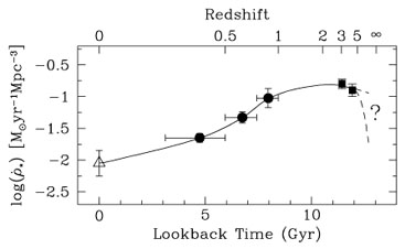
|
Figure 2. Global comoving star formation rate density vs. lookback time compiled from wide-angle ground-based surveys (Steidel et al. 1999 and references therein) assuming E-de S cosmology with h = 0.5, after Pettini (1999). Courtesy Max Pettini. |
Table 2 indicates that the known stars are
roughly accounted for by the
history shown in Fig 2 (or by Rowan-Robinson)
and the metals also if
is close to unity, i.e. the
full range of stellar masses expel
their nucleosynthesis products. At the very least,
has to be 1/2,
to account for metals in stars alone. The other point arising from the
table, made by Pettini, is that at a red-shift of 2.5, 1/4 of the stars
and metals have already been formed, but we do not know where the
resulting metals reside.
| z = 0 | z = 2.5 | |
 *
= *
=
 *(conv.) dt
| 3.6 × 10⁸
M
Mpc-3
| 9 × 10⁷
M
Mpc-3
|
 *
= * /
1.54 × 10¹¹ h702 *
= * /
1.54 × 10¹¹ h702
| .0024h70-2 | 6 × 10⁻⁴ h70-2 |
|
*(FHP 98)
| .0035h70-1 | |
|
Z
= p
*
= * /
(42
)
| 2.0 × 10⁷
M
Mpc-3
| 5 × 10⁶
M
Mpc-3
|
|
Z (predicted)
| 1.3 × 10⁻⁴
h70-2
| 3.2 × 10⁻⁵
h70-2
|
|
Z (stars,
Z = Z)
| 7 × 10⁻⁵ h70-1 | |
|
Z (hot gas,
Z =
0.3Z)
| 1.0 × 10⁻⁴h70-1.5 | |
-> 0.5  1.3
1.3
| ||
|
Z (DLA,
Z =
0.07Z)
| 2 × 10⁻⁶ h70-1 | |
|
Z (Ly. forest,
Z =
0.003Z)
| 1 × 10⁻⁶ h70-2 | |
|
Z (Ly. break gals,
Z =
0.3Z)
| ? | |
|
Z (hot gas)
| ? | |