4. EVOLUTION OF MATTER AND RADIATION FLUCTUATIONS

4.1. Damping of adiabatic fluctuations

To follow the evolution of radiation fluctuations one works with the radiation distribution function,

(4.1)

where f₀ is the blackbody distribution function, p is the photon momentum and is the photon direction. The evolution of the radiation distribution function is described by the Boltzmann equation, where the dominant interaction between radiation find matter is assumed to be Thomson scattering (Peebles and Yu, 1970; Peebles, 1980a). Neglecting possible spectral distortions one may define the frequency-averaged perturbation to the radiation brightness,

(4.2)

The direction averaged perturbation to the radiation energy density is:

(4.3)

As we discussed in Section 3, using the synchronous gauge (h₀₀ = h_i0 = 0) and decomposing the perturbation into Fourier components, the dominant mode for adiabatic perturbations on scales greater than the horizon grows as

(4.4)

in the radiation dominated era. Here _m is the Fourier transform of the fractional perturbation to the matter density _m = _m(1 + _m). When the adiabatic perturbation enters the horizon it begins to oscillate like an acoustic wave,

(4.5)

This result is valid if the matter and radiation can be treated as an ideal fluid. The mean free time for Thomson scattering is t_c = 1 / (_T n_e), where _T is the Thomson cross-section and n_e is the free electron density. Equation (4.5) thus requires t_c = 0. Whilst perturbations are in the optically thick regime we can derive an analytic estimate of the damping rate of adiabatic fluctuations as follows (Silk, 1968; Field, 1971; Chibishov, 1972; Kaiser, 1983a). If kt/a >> 1, gravity can be neglected since the scales of interest are well within the Jeans length. Assuming isotropic scattering, the equation for the radiation brightness can be written as,

(4.6a)

where µ = k ^. / |k| and is the Fourier transform of the matter velocity. The force equation for the matter is,

(4.6b)

and the equation of continuity for the matter is

(4.6c)

For a detailed derivation of these equations, including gravitational terms, see Peebles (1980a). The analysis can be further simplified if the expansion of the Universe is neglected. This is justified if the damping timescale is much shorter than the Hubble time. Equation (4.6a) may then be solved to second order in t_c,

(4.7)

where x = _r + 4 µ and k' is the proper wavenumber k' = k/a. Next we take the first moment of (4.7) and substitute into the force equation (4.6b). The zeroth moment of (4.7) gives the fluctuation in the energy density _r. Hence,

(4.8a) (4.8b)

These equations have solutions = exp(_i t), _r = exp(_i t) where,

(4.9)

where R = 1 + 3_m / 4_r (Peebles and Yu, 1970; Weinberg, 1971). If the polarizing property of Thomson scattering is included, one finds a slightly larger damping rate;

(4.10)

which exceeds _i by a factor of 4/3 in the radiation dominated limit (Kaiser, 1983a). To improve on these analytical estimates, and in particular to treat the important regime when k't_c ~ 1, one must resort to a detailed numerical solution of the Boltzmann equation (Peebles and Yu, 1970; Silk and Wilson, 1981; Wilson and Silk, 1981; Peebles, 1981a). For example, Wilson and Silk expand the angular dependence of the radiation brightness in Legendre polynomials,

(4.11)

and integrate the equations for _l(t) numerically until some time t_f when the optical depth to the observer is small. For a given wavenumber k' one requires N ~ k' t_f spherical harmonics for an accurate description. Thus for large wavenumbers, Wilson and Silk took N = 99. Alternative numerical techniques have been presented by Peebles and Yu (1970), Peebles (1981a), Kaiser (1983a) and Wyse and Jones (1983).

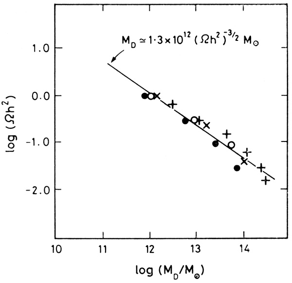Figure 4.1. Summary of results of numerical computations of the damping of adiabatic fluctuations. The damping mass is defined as MD = 44 kD-3 / 3 where kD is the wavenumber at which the transfer function takes the value 1/e. The symbols are as follows, (O) Peebles and Yu (1970), (+) Press and Vishniac (1980b), ( × ) Wilson and Silk (1981), () Peebles (1981a) (adapted from Wyse, 1982, with permission).

The results from several numerical calculations are summarized in Figure 4.1. These calculations yield a characteristic damping mass,

(4.12)

The damping process therefore results in the imposition of a characteristic feature on the fluctuation spectrum at a mass scale corresponding to groups or clusters of galaxies. Since the fluctuations are linear, each Fourier component evolves independently and so the damping effects may be summarized in terms of a linear transfer function T(k) = |_m(t_f) / _m(t_i)| where _m(t_i) is the Fourier transform of the matter density perturbation specified at some early time t_i. The transfer function is, therefore, independent of the shape of the initial fluctuation spectrum.

In Figure 4.2 we show k^3/2 |_m(t_f)| assuming an initial power-spectrum |_m|² kⁿ with n = + 1. The peaking on the largest scale, corresponding to the horizon size at decoupling, is especially prominent if = 1 since the Jeans mass is well within the horizon mass ~ 10^16.8 ( h²)^-1/2 M at decoupling. For the lower (= 0.1) case shown, there is less time for any preferential large-scale growth to occur, since the Universe only becomes matter-dominated just prior to decoupling.

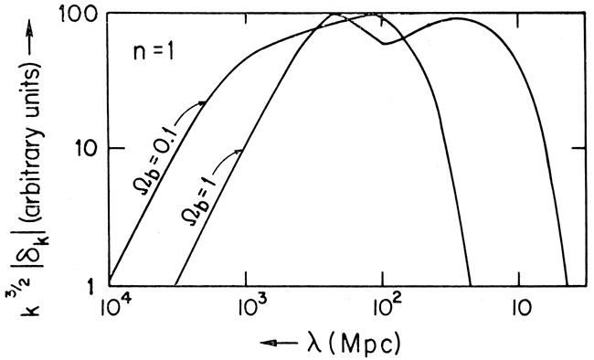Figure 4.2. Density fluctuation spectrum |k| k3/2 (contribution per unit logarithmic interval in wavenumber) as a function of comoving wavelength = 2a / k for n = 1 spectrum with H0 = 50 km sec-1 Mpc-1. Models shown are for b = 1 and 0.1, where the subscript b denotes baryons. Neutrinos are assumed to be massless in these computations. (Adapted from Wilson, 1983).

It has been argued that the drastic decrease in sound velocity at decoupling leads to supersonic compressional motions and consequently to a large amplification of adiabatic density fluctuations by up to a factor ~ 100 over galactic mass-scales (Sunyaev and Zel'dovich, 1970; Doroshkevich, Sunyaev and Zel'dovich, 1974). However, the detailed numerical studies have not shown this effect. In reality, Compton drag due to the residual ionization during decoupling strongly damps any supersonic motions, and hence there is little net amplification.