5.5.4. Empirical gas distributions derived by surface brightness deconvolution

The gas distributions in clusters can be derived directly from observations of the X-ray surface brightness of the cluster, if the shape of the cluster is known and if the X-ray observations are sufficiently detailed and accurate. This method of analysis also leads to a very promising method for determining cluster masses (Section 5.5.5). The X-ray surface brightness at a photon frequency and at a projected distance b from the center of a spherical cluster is

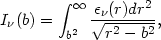
(5.80)

where is the X-ray emissivity. This Abel integral can be inverted to give the emissivity as a function of radius,

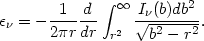
(5.81)

Because of the quantized nature of the observations of the X-ray surface brightness (photon counts per solid angle) and the sensitivity of integral deconvolutions to noise in the data, the X-ray surface brightness data are often smoothed, either by fitting a smooth function to the observations or by applying these equations to the surface brightness averaged in rings about the cluster center.

Now, the emissivity is given by equation (5.19) and depends on the elemental abundances, the density of the gas, and the gas temperature. Thus the distribution of these three properties in the cluster could be determined from observations of the X-ray surface brightness I(b). Basically, the continuum emission is due mainly to free-free emission (equation 5.11) and is relatively insensitive to the heavy element abundances, while the line emission measures these abundances. For a given set of abundances, the emissivity can be written as

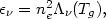
(5.82)

where (T_g) is n_p / n_e times the sum on the right side of equation (5.19). Thus (r) can be found from observations of the X-ray surface brightness as a function of photon frequency, and the frequency dependence and magnitude of give the local gas temperature and density.

Unfortunately, observations of I(b) are really not available for clusters. These observations require an instrument with good spatial and spectral resolution. Most of the X-ray spectra of clusters have been taken with instruments having very poor spatial resolution (comparable to the size of the cluster; Section 4.3.1). High spatial resolution observations of clusters have primarily come from the Einstein X-ray observatory (Section 4.4). The imaging instruments on Einstein had only limited spectral resolution. Moreover, the optics in Einstein could only focus soft X-rays (h 4 keV). At typical gas temperatures in clusters (kT_g 6 keV), most of the X-ray emissivity is due to thermal bremsstrahlung, and the emissivity is nearly independent of frequency for h kT_g. Thus the Einstein surface brightness distributions cannot be used directly to determine the local temperature. If the limited spectral resolution of the Einstein imagers is ignored, their observations provide <I_x(b)>, the surface brightness averaged over the sensitivity of the detector as a function of photon frequency.

From <I_x(b)>, the sensitivity averaged emissivity

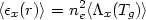
(5.83)

can be found from equation (5.81). Unfortunately, even if the elemental abundances are assumed to be known, this equation provides only one quantity at each radius, and it is impossible to determine both n_e and T_g.

In many analyses of X-ray cluster observations, a second equation for the density and temperature has been provided by assuming that the intracluster gas is hydrostatic and that the cluster potential is known. The hydrostatic equation in a spherical cluster (5.56) can be rewritten as

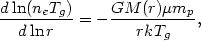
(5.84)

where m(r) is the total cluster mass and the mean atomic weight µ 0.63 is assumed to be independent of radius. Combining this with equation (5.83) gives

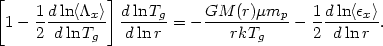
(5.85)

This is an ordinary differential equation for T_g(r), which can be integrated given a boundary condition. This has been taken to be the central temperature (White and Silk, 1980) or the intergalactic pressure (Fabian et al., 1981a). Given T_g(r), equation (5.83) gives the density profile.

Various versions of this method have been used to determine gas distributions in a large number of clusters using data from Einstein (White and Silk, 1980; Fabricant et al., 1980; Fabian et al., 1981; Nulsen et al., 1982; Fabricant and Gorenstein, 1983; Canizares et al., 1983; Stewart et al., 1984a, b). In some cases, spectral information from Einstein or low spatial resolution spectra have been used to further constrain the temperature profiles or to determine the form of the cluster potential necessary for a consistent fit (Section 5.5.5). These analyses have provided information on the mass distribution in clusters and central galaxies (M87, in particular), the gas distributions in clusters, and the prevalence of cooling accretion flows in clusters. These topics will be discussed in more detail later.

Gas temperature and density profiles could be derived more directly if high spatial and spectral resolution data at photon energies up to 10 keV were available. The proposed AXAF satellite will have these capabilities (Chapter 6).