2.2. Histograms

The oldest and most widely used density estimator is the histogram. Given an origin x₀ and a bin width h, we define the bins of the histogram to be the intervals [x₀ + mh, x₀ + (m + 1)h] for positive and negative integers m. The intervals have been chosen closed on the left and open on the right for definiteness.

The histogram is then defined by

Note that, to construct the histogram, we have to choose both an origin and a bin width; it is the choice of bin width which, primarily, controls the amount of smoothing inherent in the procedure.

The histogram can be generalized by allowing the bin widths to vary. Formally, suppose that we have any dissection of the real line into bins; then the estimate will be defined by

The dissection into bins can either be carried out a priori or else in some way which depends on the observations themselves.

Those who are sceptical about density estimation often ask why it is ever necessary to use methods more sophisticated than the simple histogram. The case for such methods and the drawbacks of the histogram depend quite substantially on the context. In terms of various mathematical descriptions of accuracy, the histogram can be quite substantially improved upon, and this mathematical drawback translates itself into inefficient use of the data if histograms are used as density estimates in procedures like cluster analysis and nonparametric discriminant analysis. The discontinuity of histograms causes extreme difficulty if derivatives of the estimates are required. When density estimates are needed as intermediate components of other methods, the case for using alternatives to histograms is quite strong.

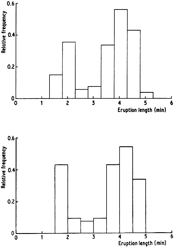
For the presentation and exploration of data, histograms are of course an extremely useful class of density estimates, particularly in the univariate case. However, even in one dimension, the choice of origin can have quite an effect. Figure 2.1 shows histograms of the Old Faithful eruption lengths constructed with the same bin width but different origins. Though the general message is the same in both cases, a non-statistician, particularly, might well get different impressions of, for example, the width of the left-hand peak and the separation of the two modes. Another example is given in Fig. 2.2; leaving aside the differences near the origin, one estimate suggests some structure near 250 which is completely obscured in the other. An experienced statistician would probably dismiss this as random error, but it is unfortunate that the occurrence or absence of this secondary peak in the presentation of the data is a consequence of the choice of origin, not of any choice of degree of smoothing or of treatment of the tails of the sample.

Fig. 2.1 Histograms of eruption lengths of Old Faithful geyser.

Fig. 2.2 Histograms of lengths of treatment of control patients in suicide study.