2.4. The kernel estimator

It is easy to generalize the naive estimator to overcome some of the difficulties discussed above. Replace the weight function w by a kernel function K which satisfies the condition

(2.2)

Usually, but not always, K will be a symmetric probability density function, the normal density, for instance, or the weight function w used in the definition of the naive estimator. By analogy with the definition of the naive estimator, the kernel estimator with kernel K is defined by

(2.2a)

where h is the window width, also called the smoothing parameter or bandwidth by some authors. We shall consider some mathematical properties of the kernel estimator later, but first of all an intuitive discussion with some examples may be helpful.

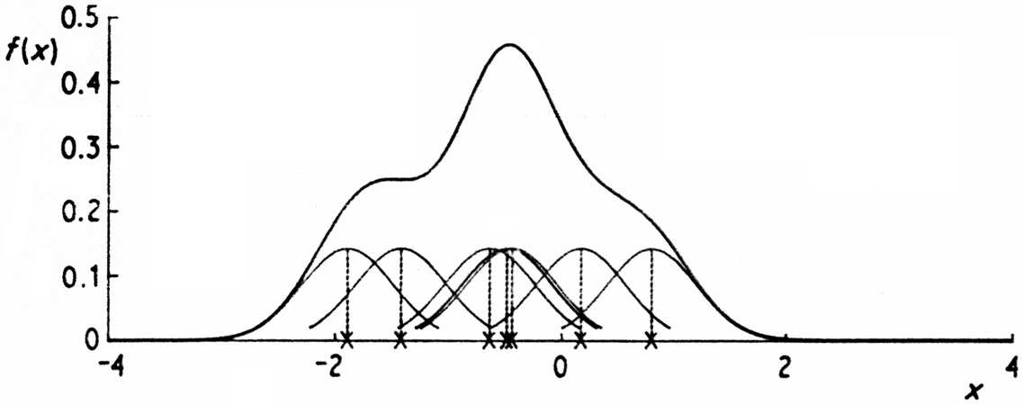
Just as the naive estimator can be considered as a sum of `boxes' centred at the observations, the kernel estimator is a sum of `bumps' placed at the observations. The kernel function K determines the shape of the bumps while the window width h determines their width. An illustration is given in Fig. 2.4, where the individual bumps n^-1 h^-1 K{(x - X_i)/h} are shown as well as the estimate constructed by adding them up. It should be stressed that it is not usually appropriate to construct a density estimate from such a small sample, but that a sample of size 7 has been used here for the sake of clarity.

Fig. 2.4 Kernel estimate showing individual kernels. Window width 0.4.

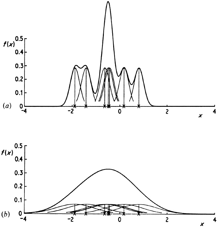
The effect of varying the window width is illustrated in Fig. 2.5. The limit as h tends to zero is (in a sense) a sum of Dirac delta function spikes at the observations, while as h becomes large, all detail, spurious or otherwise, is obscured.

Fig. 2.5 Kernel estimates showing individual kernels. Window widths: (a) 0.2; (b) 0.8.

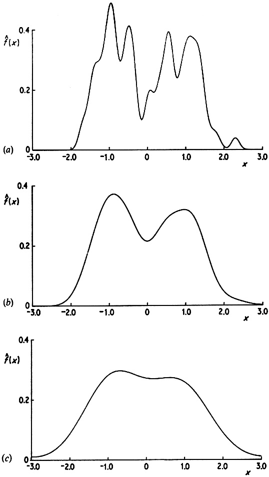
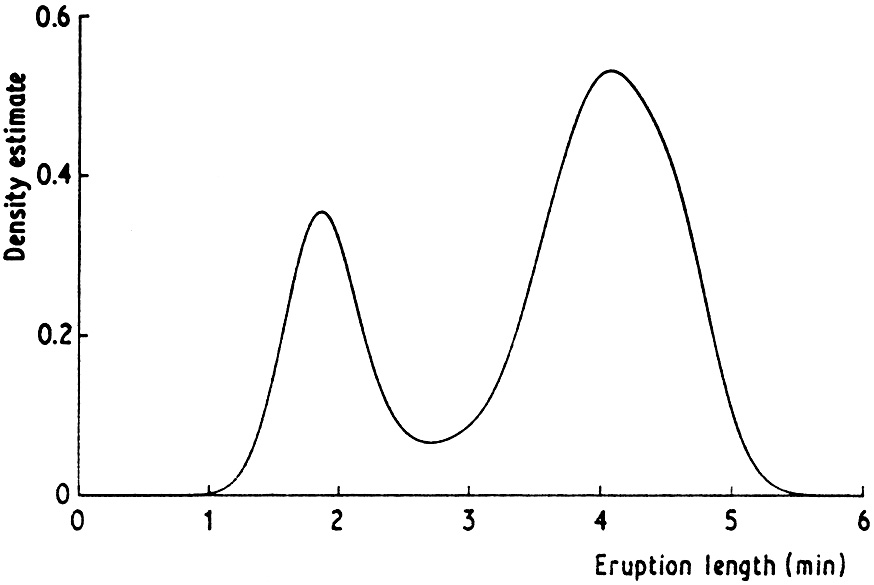
Another illustration of the effect of varying the window width is given in Fig. 2.6. The estimates here have been constructed from a pseudo-random sample of size 200 drawn from the bimodal density given in Fig. 2.7. A normal kernel has been used to construct the estimates. Again it should be noted that if h is chosen too small then spurious fine structure becomes visible, while if h is too large then the bimodal nature of the distribution is obscured. A kernel estimate for the Old Faithful data is given in Fig. 2.8. Note that the same broad features are visible as in Fig. 2.3 but the local roughness has been eliminated.

Fig. 2.6 Kernel estimates for 200 simulated data points drawn from a bimodal density. Window widths: (a) 0.1; (b) 0.3; (c) 0.6.

Fig. 2.7 True bimodal density underlying data used in Fig. 2.6.

Fig. 2.8 Kernel estimate for Old Faithful geyser data, window width 0.25.

Apart from the histogram, the kernel estimator is probably the most commonly used estimator and is certainly the most studied mathematically. It does, however, suffer from a slight drawback when applied to data from long-tailed distributions. 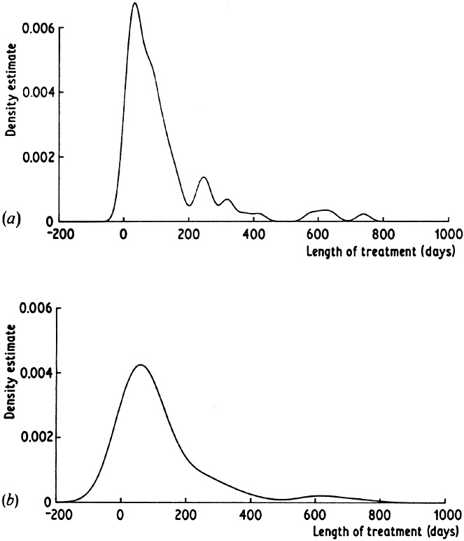Because the window width is fixed across the entire sample, there is a tendency for spurious noise to appear in the tails of the estimates; if the estimates are smoothed sufficiently to deal with this, then essential detail in the main part of the distribution is masked. An example of this behaviour is given by disregarding the fact that the suicide data are naturally non-negative and estimating their density treating them as observations on (- , ). The estimate shown in Fig. 2.9(a) with window width 20 is noisy in the right-hand tail, while the estimate (b) with window width 60 still shows a slight bump in the tail and yet exaggerates the width of the main bulge of the distribution. In order to deal with this difficulty, various adaptive methods have been proposed, and these are discussed in the next two sections. A detailed consideration of the kernel method for univariate data will be given in Chapter 3, while Chapter 4 concentrates on the generalization to the multivariate case.

Fig. 2.9 Kernel estimates for suicide study data. Window widths: (a) 20; (b) 60.