Quasar Lensing: the Observer's Point of View

3.2. Constraints and Uncertainties

Time-delays can be predicted from lens modeling, for any observed image configuration and compared with the measured ones in order to infer the value of H₀. The task requires detailed observations, deep, and at high angular resolution, and a good mass model for the lensing galaxy, as can be seen from the explicit expression for the time-delay in equations (1-3). A full description of the calculation can be found in Schneider, Ehlers & Falco (1992). We only use the result here to illustrate how observations help to achieve our goal. As explained above, the total time delay is the sum of two contributions, so that:

(1)

Each contribution to the total time-delay writes as:

(2)

(3)

where z_L is the redshift of the lensing galaxy. As illustrated in Fig. 3, the angle vector{theta} (in 2D in real cases) gives the position of the images on the plane of the sky and beta is the angular position of the source.

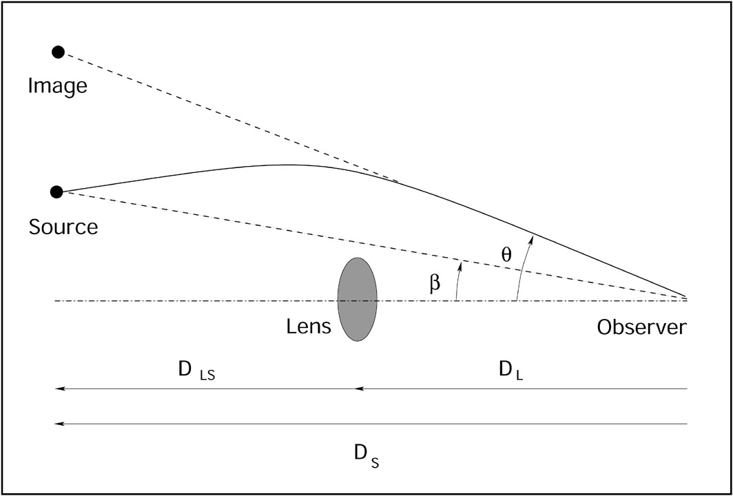Figure 3. Schematic view of a lensed quasar, with only one image represented. The difference in length between the straight (dashed) and curved (solid) lines is only responsible for the geometrical time-delay. The total time-delay also includes a gravitational part that depends on the mass distribution in the lensing galaxy (see equations 1-3).

The Hubble parameter H₀ is contained in the geometrical part of the time-delay, through the angular diameter distances to the lens D_L, to the source D_S and through the distance between the lens and the source, D_LS.

Equation (3), the gravitational part of the time-delay, depends only on well known physical constants, and on the inverse of the 2D Laplacian of the mass density profile in the lensing galaxy (). In other words, it strongly depends on the shape of the 2D mass profile of the lens (ellipticity, position angle), and on its slope. We will see later that the main source of uncertainty on the gravitational part of the time-delay comes from the radial slope of the mass distribution.

Several of the ingredients necessary to compute the time-delay can be precisely measured from observations. Although every lensed system has its own particularities, the positions of the lensed images defined by are usually the easiest quantities to constrain. With present day instrumentation, an accuracy of a few milli-arcsec is reached. The position of the lensing galaxy relative to the quasar images, when it is not double or multiple can be of the order of 10 milli-arcsec. As for the position of the source relative to the lens, it is usually free in lens models. No observation can constrain it.

In most cases, astrometry is not a major limitation to the use of lensed quasars. However, image configurations that are very symmetric about the center of the lens are more sensitive to astrometric errors than assymetric configurations. Let us assume that is very small compared with (i.e., the source is almost aligned with the lens and the observer). Lets then consider a doubly imaged quasar with two images located at positions ₁ and ₂ away from the lens, and separated by . The geometrical time-delay between the two images is:

(4)

If we now consider that the error on the image separation is much smaller than the error on the position of image 1 relative to the lens, ₁, we can approximate the error on the time-delay. Since the errors d₁ and d on ₁ and are not much correlated, they propagate on the time-delay as

(5)

In symmetric configurations, where the lens is almost midway between the images, 2|₁| ||, so that the denominator in equation (5) is zero or close to it, leading to large relative errors on the time-delay, and hence on H₀, whatever mass model is adopted for the lensing galaxy.

The advantage of symmetric configurations over assymetric ones is that they often have more than two lensed images (the source is more likely to be within the area enclosed by the radial caustic; see previous chapters on the basics of quasar lensing), offering the opportunity to measure several time-delays per system. The drawback is a larger sensitivity to astrometric errors.

Redshift information is also of capital importance in the calculation of the time-delay. Time-delays are proportional to (1 + z_L) as seen in equation (4). The angular diameter distances also depend on the redshift of the lens and source z_L and z_S. Both should therefore be measured carefully. Although the lens and source redshifts are available for most know system, their measurement is not as straightforward as one could expect. Given the small separation between the lensed images and the high luminosity contrast between the source and lens, obtaining a spectrum of the lens is often challenging and may involve significant struggling with the data (e.g., Lidman et al. 2000). In other cases, for example in systems discovered in the radio, one faces the opposite situation: the optical counterpart of the source is so faint that no spectrum can be obtained of it, while the lens is well visible (e.g., Rusin et al. 2001).

Finally, the other cosmological parameters such as Omega and Omega ₀ also play a role in the calculation of the time-delay, through the angular diameter distances. The dependence of the distances on ( Omega , Omega ₀) is however very weak. In addition, other methods (Supernovae, CMB) seem much better at pinning down their values than quasar lensing does. One shall therefore use the known values of ( Omega , Omega ₀) in quasar lensing and infer H₀, to which it is much more sensitive.