7.2. Distance indicators and methods

Direct trigonometric parallaxes that use the Earth's orbit around the Sun as a baseline for triangulation can only be used to the nearest stars. Consequently, other distance indicators and methods had to be used for extragalactic distances (see, e.g., Jacoby et al. 1992, Trimble 1997, for excellent reviews). The most common of these employ "standard candles," geometrical properties, physical properties, or various correlations to determine distances.

Standard candles are simply based on the fact that the flux of radiation decreases as an inverse square law. Objects with either a constant luminosity or whose luminosity can be related to a distance-independent measurable property (such as an oscillation period) are good standard-candle candidates. The best known and probably most reliable in this class are the Cepheid variables. Their potential as standard candles on the basis of their period-luminosity (P-L) relation was first recognized by Henrietta Leavitt in 1912, and they were used by Hubble (1925) to determine distances to Local Group galaxies. The physical processes responsible for the P-L relation are broadly understood. Near ionization zones (in this case, primarily He⁺ He⁺⁺), gas can absorb heat under compression and release it after maximum compression. This leads to an instability strip in the effective temperature-luminosity plane, which, in the case of Cepheids, is very narrow in temperature. The pulsation period depends on the mass and radius as

(25)

The luminosity of the star (which is determined ultimately by nuclear reactions that depend on the density and temperature) is proportioned to a power of the mass, L ~ M^k. Since, however, we also have (for black body radiation) L ~ R² T⁴, we obtain P ~ L^{(3 k + 2)/4} T^-3, or a period-luminosity-color relation. One of the "Key Projects" of HST has been to measure H₀ based on a Cepheid calibration of a number of secondary distance determination methods.

The results of this project have been described in a series of some 30 papers (see Freedman et al. 2001, and references therein). The main goals of the project have been: (i) To discover Cepheids in a sample of relatively nearby galaxies (with distances 20 Mpc) and to determine distances to these galaxies. (ii) To determine H₀ through several secondary distance indicators, to all of which Cepheid calibration is applied; and perhaps most importantly, (iii) To determine the uncertainties in all the methods by comparing the distances obtained from them to Cepheid-based distances. As a part of the project, the uncertainties in the Cepheid P-L relation itself (and its dependence on other factors such as metallicity) have been investigated.

The Key Project used Cepheid calibration to 31 galaxies, of which 18 have been observed and analyzed in the context of the project, and to which archival data, and data on the nearby galaxies M31, M33, IC 1613, NGC 300, and NGC 2403 have been added.

The Key Project used the following secondary methods based on Cepheid distances: Type Ia Supernovae, the Tully-Fisher Relation, the Fundamental Plane for elliptical galaxies, Surface Brightness Fluctuations and Type II Supernovae. Let me describe very briefly the physical basis for each one of these methods.

7.2.1. Type Ia supernovae

Type Ia supernovae at peak brightness are extremely bright, with M_B M_V - 19.3 + 5 log(H₀/60), and they show a relatively low dispersion, (M_B) ~ 0.33 (e.g., Branch 1998). Furthermore, there exists a relatively tight correlation between their peak luminosity and light-curve shape (or rate of decline, with brighter supernovae declining more slowly; Phillips 1993, Hamuy et al. 1996, Riess et al. 1996). The homogeneity may be related to the fact that Type Ia supernovae represent thermonuclear disruptions of mass-accreting white dwarfs, when the latter reach the Chandrasekhar limit (e.g., Livio 2001). The luminosity-light-curve relation may be the result of the following (e.g., Arnett 2001). The peak luminosity of a supernova Type Ia is proportional to the mass of ⁵⁶Ni that is produced. A higher mass of ⁵⁶Ni, however, also results in more heating and concomitantly a higher opacity (due mainly to UV lines). Consequently, a slower development of the light curve results.

7.2.2. The Tully-Fisher relation

For spiral galaxies, that are known to have flat rotation curves, there is an observationally-determined relationship (Tully and Fisher 1977) between the total luminosity and the maximum rotational velocity (both corrected for inclination effects), of the form L ~ V³_max (in the I band). The scatter around this relation is about ±0.3 mag (e.g., Giovanelli et al. 1997).

There is no precise physical understanding of the Tully-Fisher relation. Very broadly, a similar relation can be obtained from the following argument (e.g., Eisenstein and Loeb 1996). Consider a galaxy (of mass M) collapsing from a spherical cloud. At epoch t_coll, the turnaround radius R_t is

(26)

After virialization, the energy is

(27)

where is the velocity dispersion. Combining the above and assuming that the galaxy forms from a single collapse gives

(28)

Therefore, if all galaxies collapse at the same epoch and the mass-to-light ratios, M/L, do not vary significantly, we obtain L ~ ³.

7.2.3. The fundamental plane for elliptical galaxies

Large spectrophotometric surveys conducted during the mid-1980s (e.g., Djorgovski and Davis 1987, Dressler et al. 1987) revealed that, for elliptical galaxies, a tight correlation exists between the effective radius, R_e, the effective surface brightness, SB_e, and the central velocity dispersion , of the form (the "fundamental plane")

(29)

Here R_e is in kpc, in km s^-1, and SB_e in mag arcsec^-2. The value of depends on H₀, since the calculation of the effective radius in kpc uses the Hubble constant.

The physical origin of the fundamental plane relation can be understood on the basis of the following simple considerations (e.g., Treu et al. 2001). We can define an effective (virial) mass by

(30)

Let us also assume that the mass-to-light ratio satisfies

(31)

We then obtain

(32)

which reduces to the fundamental plane relation for reasonable values of ( ~ 0.25).

7.2.4. Surface brightness fluctuations

The method of surface brightness fluctuations was developed by Tonry and Schneider (1988) and Tonry et al. (1997, 2000). The method basically makes use of the obvious fact that the ability to resolve stars within galaxies is distance dependent. More specifically, for every region of a galaxy one can measure the average flux per pixel, g, and the pixel-to-pixel rms, . Since the flux obtained in a pixel is received from N stars of average flux , we have g = N and = N^1/2 . A galaxy which is twice as distant appears twice as smooth as the closer galaxy. Consequently, the average stellar flux is given by = ² / g (and scales as the inverse of the square of the distance).

7.2.5. The Expanding Photosphere Method of Type II supernovae

Type II supernovae result from the collapse of stars more massive than about 8 M. Generally, Type II supernovae are fainter than Type Ia supernovae, and they also exhibit a considerably larger range in their luminosities, making them poorer standard candles. Nevertheless, Type II supernovae have been used as distance indicators, through an application of the Expanding Photosphere Method (e.g., Kirshner and Kwan 1974, Schmidt et al. 1994).

The basic idea is simple. The angular size of the photosphere is given by (for z << 1)

(33)

where T is the color temperature, f is the flux density, B(T) is the Planck function, and represents the dilution effects of scattering atmospheres (derived from model atmospheres).

The photospheric radius is given by

(34)

where v is the expansion velocity (measured from the absorption minima of optically thin lines), and the initial radius, R_o, can be neglected at all but the earliest times. Combining the above yields

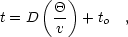(35)

making it possible to determine both the distance and the time of the explosion from a few measurements of t, v, .