Probing the Universe with Weak Lensing

Annu. Rev. Astron. Astrophys. 1999. 37: 127-189
Copyright © 1999 by Annual Reviews. All rights reserved

2. DEFINITIONS

In this preliminary section, I do not discuss at length the theoretical basis of the gravitational lens effect because all the details can be found in the comprehensive textbook written by Schneider et al (1992). I focus on concepts and basic equations of the gravitational lensing theory, in the thin lens approximation and for small deviation angles, which are necessary for this review.

The apparent angular position of a lensed image, theta ^I (in this review, bold symbols denote vectors), can be expressed as a function of the (unlensed) angular position of the source, theta ^S, and the deflection angle, alpha ( theta ^I) as follows (see Figure 1):

$\begin{equation} \thetag^I=\thetag^S+{D_{LS} \over D_{OS}} \alphag(\thetag^I) \ . \end{equation}$

(1)

alpha ( theta ^I). depends on the projected mass density of the lens, Sigma ( theta ^I), and the cosmological parameters through the angular-diameter distances from the lens L to the source S, D_LS, from the observer o to the source, D_OS, and from the observer to the lens, D_OL:

$\begin{equation} \alphag(\thetag^I)={4 \pi G \over c^2}D_{OL} \ \ {1 \over \pi} \int \Sigma(\thetag^I) {\thetag^I - \thetag' \over \vert \thetag^I - \thetag' \vert^2} d^2\theta' \ . \end{equation}$

(2)

where G is the gravitational constant and c is the speed of light. Sigma ( theta ^I) can be expressed as a function of the Poisson equation, and the strength of the lens is characterized by the ratio of the projected mass density of the lens to its critical projected mass density Sigma _crit (see Fort & Mellier 1994):

$\begin{equation} {\Sigma(\thetag^I) \over \Sigma_{crit}}= {4 \pi G \over c^2}{D_{LS}D_{OL}\over D_{OS}} \Sigma(\thetag^I)={1 \over 2} \Delta \varphi(\thetag^I) \end{equation}$

(3)

where Delta is the 2-dimension Laplacian and phi is the dimensionless gravitational potential projected along the line of sight which is related to the projected gravitational potential Phi as follows:

$\begin{equation} \varphi={2 \over c^2} \ {D_{LS}D_{OL}\over D_{OS}} \Phi \ . \end{equation}$

(4)

From the differentiation of Equation (1), we can express the deformation of an infinitesimal ray bundle as a function of the Jacobian

$\begin{equation} { d \thetag^S \over d \thetag^I}=A(\thetag^I) \ , \end{equation}$

(5)

where A( theta ^I) is the magnification matrix:

$\begin{equation} \begin{equation} A=\left( \begin{array}{cc} 1-\partial_{11} \varphi & -\partial_{12} \varphi \\ -\partial_{12} \varphi & 1-\partial_{22} \varphi \\ \end{array} \right) \end{equation}$

(6)

It can be written as a function of two parameters (similar to the magnification and the astigmatism terms in classical optics), the convergence, kappa , and the shear components gamma ₁ and gamma ₂ of the complex shear gamma = gamma ₁ + i gamma ₂:

$\begin{equation} A=\left( \begin{array}{cc} 1-\kappa-\gamma_1 & -\gamma_2 \\ -\gamma_2 & 1-\kappa+\gamma_1 \\ \end{array} \right) \end{equation}$

(7)

The isotropic component of the magnification, kappa = 1/2 Delta phi ( theta ^I), is directly related to the projected mass density, and the two components gamma ₁ and gamma ₂ describe an anisotropic deformation produced by the tidal gravitational field. The eigenvalues of the magnification matrix are 1 - kappa ± | gamma |, where | gamma | = ( gamma ₁² + gamma ₂²)^1/2. They provide the elongation and the orientation produced on the images of lensed sources. The magnification of an image is:

$\begin{equation} \mu = {1 \over det(A)} = {1 \over (1-\kappa)^2-\vert \gammag \vert^2} \ . \end{equation}$

(8)

The points of the image plane where det (A) = 0 are called the critical lines. The corresponding points of the source plane are called the caustic lines and produce infinite magnification (see Schneider et al 1992;, Blandford & Narayan 1992;, Fort & Mellier 1994 for more detailed descriptions of caustic and critical lines). The strong lensing cases correspond to configurations where sources are close to the caustic lines. These lenses have Sigma ( theta ^I) / Sigma _crit geq 1 and the convergence and shear are strong enough to produce giant arcs and multiple images for suitably positioned sources (Figures 2 and 3). The weak lensing regime, which is the main topic of this review, corresponds to lensing configurations where kappa << 1 and gamma << 1. In this regime, the magnification and the distortion of background galaxies are so small that they cannot be detected on individual objects. In that case, it is necessary to analyze statistically the distortion of the lensed population.

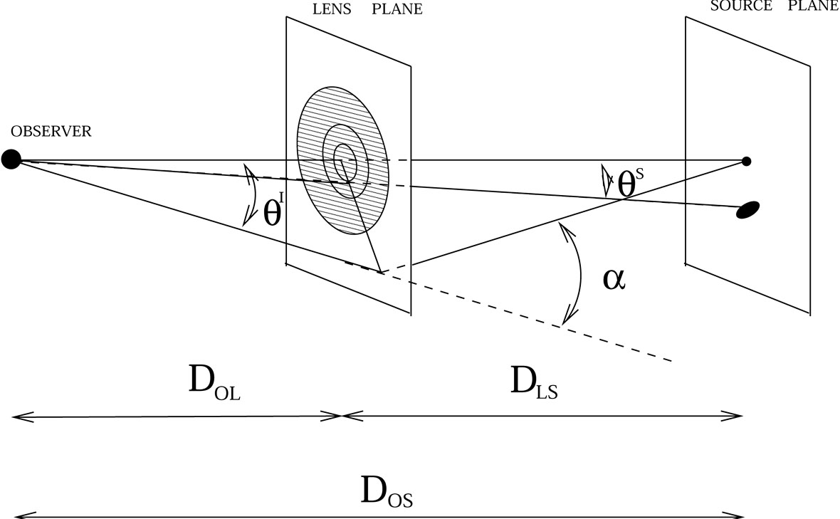Figure 1. Description of a lensing configuration.

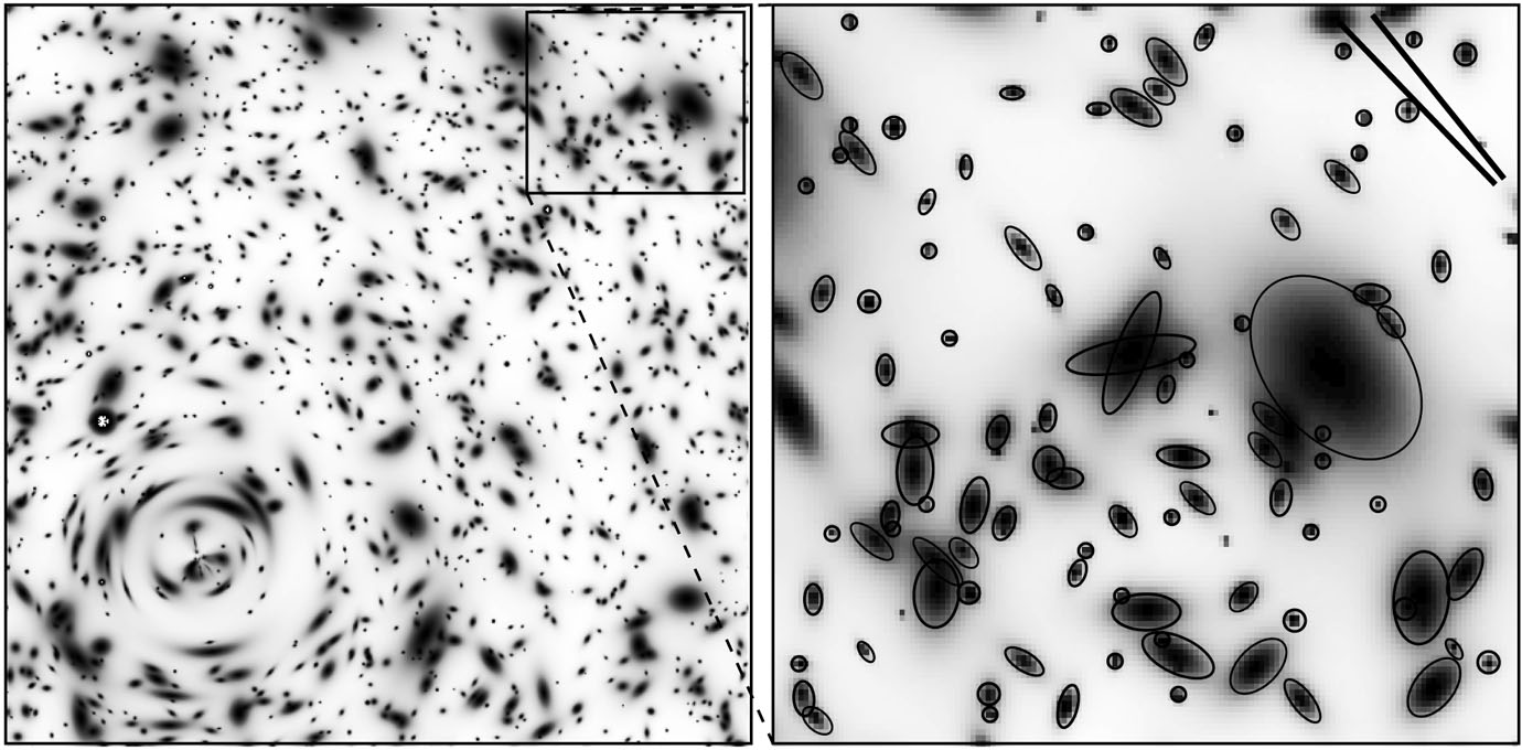Figure 2. Illustration of the two lensing regimes. The left panel is a simulation of a cluster of galaxies at redshift 0.15, modeled by an isothermal sphere with a velocity dispersion of 1300 km s^-1. The lensed population has an average redshift of one. In the innermost region (bottom left part of the panel), tangential and radial arcs are clearly identified. As the radial distance of lensed galaxies increases, the shear decreases, and far from the cluster center, the ellipticity produced by the shear is lower than the intrinsinc ellipticity of the galaxies. The lensing signal must be averaged over a large number of galaxies in order to be measured accurately. The zoom on the right panel shows the images of the galaxies in the weak lensing regime. The contours show their shape as determined from their second moments. The average orientation of these galaxies is given by the solid lines at the top right. The lower line is the true orientation of the shear produced by the cluster at that position and the upper line is the orientation computed from 92 galaxies of the zoomed area. The difference between the two orientations is random noise due to the intrinsinc ellipticity and orientation distributions of the galaxies.

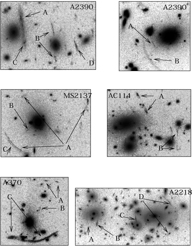Figure 3. A panel of lensing clusters observed with HST. The arc(let)s and multiple lensed images are indicated by a letter. In A2390 (top left), the straight arc is made of two different galaxies corresponding to images A and C. The pairing of some images is obvious, like B in A2390 (top-left), A in AC114, or A in A370. Image B in MS2137 and B in A370 are radial arcs. A in MS2137 is a triple image from an almost ideal configuration of a fold caustic.