


The standard model for describing the global evolution of the Universe is based on two equations that make some simple, and hopefully valid, assumptions. If the Universe is isotropic and homogenous on large scales, the Robertson-Walker Metric,
 |
(4) |
gives the line element distance(s) between two objects with coordinates
r,  and time separation, t. The Universe is assumed to have a simple
topology such that, if it has negative, zero, or positive curvature,
k takes the value
-1, 0, 1, respectively. These models of the Universe are said to be
open, flat,
or closed, respectively. The dynamic evolution of the Universe needs to be
input into the Robertson-Walker Metric by the specification of the scale
factor a(t),
which gives the radius of curvature of the Universe over time - or more
simply, provides the relative size of a piece of space at any time. This
description of the dynamics of the Universe is derived from General
Relativity, and is known as the Friedman equation
and time separation, t. The Universe is assumed to have a simple
topology such that, if it has negative, zero, or positive curvature,
k takes the value
-1, 0, 1, respectively. These models of the Universe are said to be
open, flat,
or closed, respectively. The dynamic evolution of the Universe needs to be
input into the Robertson-Walker Metric by the specification of the scale
factor a(t),
which gives the radius of curvature of the Universe over time - or more
simply, provides the relative size of a piece of space at any time. This
description of the dynamics of the Universe is derived from General
Relativity, and is known as the Friedman equation
 |
(5) |
The expansion rate of our
Universe (H), is called the Hubble parameter (or the
Hubble constant, H0, at the present epoch) and
depends on the
content of the Universe. Here we assume the Universe is composed of a
set of components, each having a fraction,
 i, of the
critical density
i, of the
critical density
 |
(6) |
with an equation of state which relates the density,
 i,
and pressure, pi, as
wi = pi /
i.
For example, wi takes the value 0 for normal
matter, +1/3 for photons, and -1 for
the cosmological constant. The
equation of state parameter does not need to
remain fixed; if scalar fields are present, the effective w will
change over time. Most reasonable forms of matter or scalar fields have
wi
i,
and pressure, pi, as
wi = pi /
i.
For example, wi takes the value 0 for normal
matter, +1/3 for photons, and -1 for
the cosmological constant. The
equation of state parameter does not need to
remain fixed; if scalar fields are present, the effective w will
change over time. Most reasonable forms of matter or scalar fields have
wi  - 1,
although nothing seems manifestly
forbidden. Combining Eqs. (4-6) yields solutions to
the global evolution of the Universe
[13].
- 1,
although nothing seems manifestly
forbidden. Combining Eqs. (4-6) yields solutions to
the global evolution of the Universe
[13].
The luminosity distance, DL, which is defined as the apparent brightness of an object as a function of its redshift z - the amount an object's light has been stretched by the expansion of the Universe - can be derived from Eqs. (4-6) by solving for the surface area as a function of z, and taking into account the effects of time dilation [25, 26, 50, 82] and energy dimunition as photons get stretched traveling through the expanding Universe. DL is given by the numerically integrable equation,
 |
(7) |
S(x) = sin(x), x, or sinh(x) for closed,
flat, and open models respectively, and the curvature parameter
 0, is
defined as 0 =
0, is
defined as 0 =
 i
i - 1.
i
i - 1.
Historically, Eq. (7) has not been easily integrated and has been expanded in a Taylor series to give
 |
(8) |
where the deceleration parameter, q0, is given by
 |
(9) |
From Eq. (9) we can see that, in the nearby Universe, the
luminosity distances scale linearly
with redshift, with H0 serving as
the constant of proportionality. In the more distant Universe,
DL
depends to first order on the rate of acceleration/deceleration
(q0) or,
equivalently, on the amount and types of matter that make up the Universe.
For example, since normal matter has wM = 0 and the
cosmological constant has
w = - 1, a universe composed of only these two forms of
matter/energy has q0 =
M / 2 -
. In a universe
composed of these two types of matter, if
<
M / 2,
q0 is positive and the universe is
decelerating. These decelerating
universes have DL smaller as a function of z
than their accelerating counterparts.
= - 1, a universe composed of only these two forms of
matter/energy has q0 =
M / 2 -
. In a universe
composed of these two types of matter, if
<
M / 2,
q0 is positive and the universe is
decelerating. These decelerating
universes have DL smaller as a function of z
than their accelerating counterparts.
If distance measurements are made at a low-z and a small range of
redshift at higher z (e.g., 0.3 > z > 0.5),
there is a degeneracy between
M and
. It is
impossible to pin down
the absolute amount of either species of matter. One can only determine
their relative dominance, which, at z = 0, is given
by Eq. (9). However, Goobar and Perlmutter
[27]
pointed out that
by observing objects over a larger range of high redshift (e.g.,
0.3 > z > 1.0) this
degeneracy can be broken, providing a measurement of the absolute
fractions of
M and
.
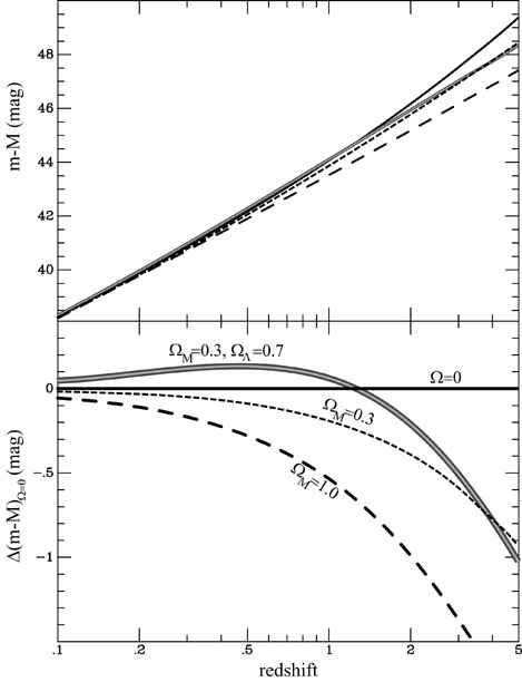 |
Figure 1. DL expressed as
distance modulus (m - M) for four relevant cosmological
models;
|
To illustrate the effect of cosmological parameters on the luminosity
distance, in Fig. 1 we plot a series of
models for both
and non- universes.
In the top panel, the various models show the same linear behavior at
z < 0.1 with
models having the same H0 being indistinguishable to a
few percent. By z = 0.5 the models with significant
are clearly
separated, with luminosity distances that are significantly further than the
zero- universes.
Unfortunately, two perfectly reasonable universes, given our knowledge
of the local matter density of the Universe
(M ~
0.2), one with a large cosmological constant,
= 0.7,
M = 0.3
and one with no cosmological constant,
M = 0.2,
show differences of less than 25%, even to redshifts of z >
5. Interestingly, the maximum difference between the two models is at
z ~ 0.8, not at
large z. Fig. 2
illustrates the effect of changing the equation of state of
the non-matter, dark energy component, assuming a flat universe,
tot =
1. If we are to discern a dark energy component that is not a
cosmological constant, measurements better than 5% are clearly required,
especially since the differences in this diagram include the assumption of
flatness and also fix the value of
M. In
fact, to discriminate
among the full range of dark energy models with time varying equations
of state will require much better accuracy than even this challenging goal.
 |
Figure 2. DL for a
variety of cosmological models containing
|