2.5. Dissipative Gravitational Settling

Dissipative settling has increased the magnitude of the gravitational binding energy from that prescribed by the primeval conditions considered in the last section. In Section 2.5.1 we discuss the energy released in producing the increased mean density of baryons relative to dark matter in the luminous parts of the galaxies, in Section 2.5.2 we estimate the gravitational energy released in stellar formation and evolution, and in Section 2.5.3 we consider the central massive compact objects in galaxies.

2.5.1. The Luminous Parts of Galaxies

In the Milky Way galaxy the mass within our position, at about 8 kpc from the center, is roughly equal parts baryonic and dark matter, or about 6 times the cosmic mean ratio (eq. [18]). This is thought to be the usual situation in the luminous parts of normal galaxies. The amount of gravitational binding energy released in producing this concentration of baryons depends on how it was done. In one limiting case one may imagine that stars formed in the centers of low mass dark halos with relatively small dissipation of energy - apart from star formation - because the depths of the gravitational potential wells were small, and that the low mass halos later merged without any additional dissipation, the dense baryon-dominated parts remaining near the densest regions to form the present-day baryon-dominated luminous parts of galaxies. (This is an extreme version of the scenario discussed by Gao et al. 2003). In another extreme, one may imagine that the baryons settled into previously assembled galaxy-scale halos, which would dissipate considerably more energy. A galaxy has a definite computable gravitational binding energy, of course (apart from the difficulty of correcting for ongoing accretion), but to relate this to the energy dissipated in producing the galaxy would require an analysis of what the mass distribution would have been in the absence of dissipation, which is not an easy task.

These considerations lead us to offer only a crude estimate for entry 5.1, which we write as the product of the density parameter belonging to baryons in galaxies - the sum _{b, g} = 0.0035 of the density parameters in entries 3.3 to 3.13 - with the kinetic energy per unit mass, K = 3² / 2 and = 160 km s^-1. The result is a 2% addition to the primeval halo gravitational binding energy (entry 4.1). If the baryon concentrations in galaxies formed at high redshifts in small halos the dissipative energy released would be an even smaller fraction of the total.

2.5.2. Stellar Binding Energy

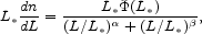
The amount of binding energy released in star formation is easy to define because the relative length scale is small. We write the gravitational binding energy per unit mass for a star with mass m and radius r as

(68)

The prefactor for the Sun is K = 1.74, and K = 0.3 for a homogeneous sphere.

For main sequence stars we use the zero-age mass-radius relation, r 0.85 m^0.80 for 0.08 < m < 0.79, r 0.93 m^1.17 for 0.79 < m < 1.38, and r 1.15 m^0.52 for 1.38 < m < 100, in solar units. These numbers are assembled from Ezer & Cameron (1967), Cox & Giulli (1968) and Cox (2000). Integration of Gm² / r over the PDMF gives BE / m = 3.7 × 10^-6. The product of the last number with the density parameter of the mass in main sequence stars (entries 3.3 plus 3.4), with K K, is the estimate of the gravitational binding energy, _BE = - 10^-8.1, for stars. We similarly obtain the substellar gravitational binding energy, _BE = - 10^-9.6, where r is fixed at 0.096 r (Burrows et al. 2001). This is a small addition to the sum in entry 5.2.

We construct a model for the white dwarf mass function from an approximation to the relation between the progenitor main sequence mass and the white dwarf remnant mass (Claver et al. 2001; Weidemann 2000),

(69)

and our PDMF. White dwarf masses run from 0.53 to 1.09 m for the main sequence mass range 1 < m_ms < 8 m we have adopted. The white dwarf mass function dN / dm_wd = (dN / dm_ms)(dm_ms / dm_wd) thus obtained agrees well with the observed white dwarf mass distribution of Bergeron & Holberg (in preparation). In our mass function the mean white dwarf mass is

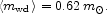(70)

From our mass function and the mass-radius relation given by Shapiro and Teukolsky (1983) we obtain the mean white dwarf gravitational binding energy per unit mass,

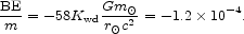(71)

Since the fractional half-mass radius of a white dwarf is 0.57 times the solar value (Schwarzschild 1958), we have taken K_wd 1.0. The product with the mass density in white dwarfs (entry 3.5) is entry 5.3.

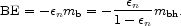
We take the binding energy of a neutron star to be 3 × 10⁵³ erg (e.g., Burrows 1990; Janka & Hillebrandt 1989), or

(72)

The product with entry 3.6 is entry 5.4. This is the largest among all gravitational binding energies in the inventory.

2.5.3. Black Hole Binding Energy

Our definition of the binding energy associated with a black hole requires careful explanation because it has some curious properties, including violation of the thought that it would be logical to consider the mass of a black hole to be purely gravitational if the matter out of which it formed has lost its existence.

We choose the definition by analogy to nuclear and Newtonian gravitational binding energy, in terms of the energy liberated in the assembly of a system out of its initial parts, that is, the difference between the total mass of the initial parts and the mass of the assembled system. In the same way, we use equations (49) and (50) to define the binding energy of a black hole by the difference between the mass m_b of the initial parts - baryons - and the mass m_bh = (1 - _n) m_b of the final black hole. Thus our definition of the binding energy of a black hole is

(73)

The magnitude of BE is the energy emitted as electromagnetic and gravitational radiation, neutrinos, and kinetic energy, as is appropriate for our purpose of telling the energy transfers and balancing the baryon budget. It will be noted that in this definition the binding energy depends on how the black hole formed. For example, a Solar mass black hole that formed with efficiency = 0.99 is assigned binding energy -99 m, because it released that much energy, while an identical black hole that formed with _n = 0.01 is assigned a very different binding energy, -0.01 m.

Entry 5.5 for the gravitational binding energy of stellar mass black holes is the product of entry 3.7, which is our estimate of the baryonic mass entering the black hole, with the efficiency factor _s. In the standard picture for the formation of a stellar mass black hole, a core of baryons is first burned to heavy elements, and the subsequent collapse to a black hole may release little more energy. In this case the efficiency factor could be as small as _s ~ 0.009, which is the binding energy released as starlight. It could also be as large as _s ~ 0.03 if the collapse proceeded through a protoneutron star as an intermediate state. It cannot be much larger, however, without violating the constraints from the radiation energy density (see Section 2.7) and the relic supernova neutrino flux at Super-Kamiokande (Fukugita & Kawasaki 2003).

One way to estimate the mass density in the massive black holes in the nuclei of galaxies uses the correlation of the black hole mass with the bulge luminosity. A convenient approximation to the relation, for B-band luminosities, is (Gebhardt et al. 2000; Ferrarese 2002; see also Kormendy & Richstone 1995)

(74)

FHP estimate that the fraction of the B-band luminosity density in ellipticals and S0 galaxies is 0.24, and the fraction in the bulges of spheroids is 0.14. The products of equation (74) with the luminosity fractions and the luminosity density in equation (21) gives the mass density parameters in massive black holes,

(75)

Salucci et al. (1999) give a consistent, but slightly larger value.

For early-type galaxies we can use the tight relation between the black hole mass and the bulge or spheroid velocity dispersion (Merritt & Ferrarese 2001; Tremaine et al. 2002). The Sheth et al. (2003) estimate of the velocity dispersion function for early-type galaxies is

(76)

with = 6.5, = 1.93, _* = 89 km s^-1, _* = 0.0020 Mpc^-1. The Tremaine et al. (2002) estimate of the black hole mass-velocity dispersion relation is

(77)

with B = 1.3 × 10⁸ m, a = 4.0, and _h = 200 km s^-1. The product of the two expressions, integrated over , gives the mean mass density,

(78)

The numerical result,

(79)

is close to but smaller than the more direct estimate in equation (75). Although the formal uncertainty in equation (79) is smaller it rests on the condition that the Sheth et al. galaxies are a fair sample of the early-type galaxies, which will require careful debate. ⁶ Thus in the inventory we quote equation (75).

Soltan (1982) and Chokshi & Turner (1992) have considered the relation between the rate of radiation of energy by quasars and AGNs and the accumulation of mass in the quasar engines, which are assumed to be massive black holes in the centers of galaxies. In this repetition of the calculation we take the number of quasars per unit luminosity and comoving volume to be

(80)

where, from Croom et al. (2004), = 3.31, = 1.09,

(81)

the present b_J characteristic luminosity is

(82)

and the characteristic luminosity at z = 2 is 42 times this value. The integral dL L dn / dL is the comoving luminosity density, and the time integral multiplied by the bolometric correction factor (BC = 12.2, according to Elvis et al. 1994) is the energy density released. We assume pure luminosity evolution, with the variation of L_* with redshift given by the Croom et al. (2004) polynomial model to redshift z = 2.1. This is the deepest redshift used in their analysis. Since the comoving density of the most luminous quasars decreases at higher redshifts, we assume the comoving luminosity density is constant from z = 2.1 to z = 3 and is negligibly small at larger redshifts. In this model the integrated energy density released is = 1.4 × 10^-7. If the efficiency _n for energy production is small the estimate of the integrated mass added to the massive black holes by the observed quasars and AGNs is then

(83)

The ratio of this number to the mass density in massive black holes (the sum of entries 5.6 and 5.7) is an estimate of the radiation efficiency,

(84)

This is not very far from the commonly discussed value, _n ~ 0.1. A closer check of consistency with the idea that the massive black holes are the quasar remnants awaits advances in the measurements of the luminosity function for fainter objects and larger redshifts.

⁶ The velocity function of Sheth et al. gives <⁴>^1/4 = 180 km s^-1, compared to our estimate of the characteristic velocity dispersion, _* = 200 - 220 km s^-1, in early-type galaxies. Perhaps this is related to the difference. Back.