G. The cosmic microwave background

The importance of the CMB anisotropy measurements cannot be over-emphasized and would warrant an entire review by itself. From the point of view of this article we are concerned with knowing the initial conditions for galaxy formation and the parameters of the cosmological framework within which galaxy formation takes place. Given that data, the task is to derive the currently observed clustering properties of galaxies in the Universe.

1. Structure before our eyes

Arguably the most important observation in the study of clustering is the recent measurement of the structure in the cosmic microwave background radiation at the time of recombination. This structure was predicted independently by Silk (1967) and by Sachs and Wolfe (1967), although the phenomenon is generally referred to as the "Sachs-Wolfe" effect. Understanding the details of how the structure in the microwave background arises in any of a vast number number of cosmological models has been a cosmic folk-industry spanning some 30 years. The results are encapsulated in a run-it-yourself computer program of Zaldarriaga and Seljak, 2000 (see http://physics.nyu.edu/matiasz/CMBFAST/cmbfast.html).

The structure was first seen at about 7° in angular resolution in the data of the COBE satellite DMR experiment (Bennett et al. 1996). Smaller structure has been detected in recent high angular resolution experiments with names like DASI (Leitch et al., 2002; Pryke et al., 2002), MAXIMA-1 (Hanany et al., 2000; Lee et al., 2001; Balbi et al., 2000) and BOOMERANG-98 (de Bernardis et al., 2000; Lange et al., 2001; Netterfield et al., 2002), and in the WMAP first-year full-sky data (Bennett et al., 2003). An analysis of the cosmological conclusions to be drawn from the combination of these is given by Jaffe et al. (2001) and by Spergel et al. (2003); an example of present data sets and the curves fitted to them is shown in Fig. 8 where, in addition to the WMAP power-spectrum, several other recent experiments are shown (VSA analyzed by Dickinson et al. (2004), CBI (Mason et al., 2003) and ACBAR (Kuo et al., 2004), having similar sensitivity, but being different in the frequency range and observing techniques.

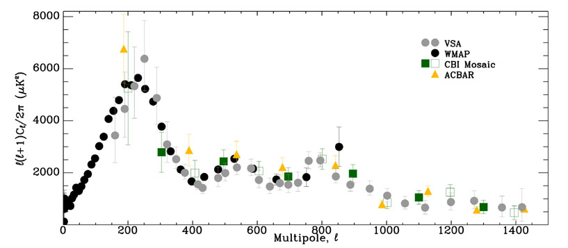Figure 8. The agreement between the estimated power spectrum of the CMB anisotropies from four different experiments with similar sensitivity, from Dickinson et al. (2004).

The units in Fig. 8 could use a little bit of explanation. As the sky we see can be thought of as a surface of a sphere, the distribution of temperature on the sky is analysed into scales using Legendre polynomials Y_l^m(, ). A polynomial of order l picks out structure on an angular scale that is roughly, in degrees,

(6)

This corresponds to structure on a linear scale today of

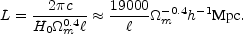(7)

for a flat universe with _m + = 1 (Vittorio and Silk, 1992). The range of l-values covered by current experiments range over about two decades:

(8)

with the limit of higher l-values being pushed upward all the time. The low resolution end is from the COBE and WMAP data (Bennett et al., 1996; Bennett et al., 2003) and reveals inhomogeneities on scales in excess of 100h^-1 Mpc.

Notice that the highest resolution data still only cover linear scales in excess of around 30 h^-1 Mpc and so we do not yet see the initial condition for the scales over which the two-point galaxy clustering correlation function is significantly greater than zero. We are just seeing the scales where rich cluster clustering may be significant. The prominent peak in the spectrum at l ~ 250 corresponding to scales of around 50 h^-1 Mpc is intriguing. We must not forget, however, that this is a peak in a normalized spectrum; in the real matter P(k) these peaks are much less pronounced. There is evidence of oscillations in the observed power spectra of clusters and galaxies, but current surveys are not able yet to detect such structure with confidence (Miller et al., 2002a; Elgarøy et al., 2002).

2. Defining the standard model

The presence of significant peaks in the angular distribution of the cosmic microwave background strongly constrains the global parameters that describe our Universe. If these data are combined with data from other sources, such as local determinations of the Hubble constant and observations of very distant supernovae (Riess et al., 1998; Perlmutter et al., 1999), we arrive at the so-called concordance model (Tegmark et al., 2001). We hasten to add that this is not a term we invented: it might have been OK to use the term standard model, but the high energy physicists got there first. The actual values of the parameters in the concordance model depends on whose paper we read: there is a little disaccord here, though it would seem to be relatively minor. It all depends on what prior knowledge is assumed when making fitting the model to the data. The error bars are impressively small.

3. Initial conditions for galaxy formation

One of the best determined parameters is the slope n of the power spectrum of the pre-recombination inhomogeneities. It was suggested by Harrison and by Zel'dovich that n = 1 on the grounds that (a) the spectrum had to be a power law (what else could it be?) and that (b) this value of the slope was the value that did the minimal violence to the geometry of space-time on either the large or small scales. Following on Guth's brilliant notion of inflationary cosmology (Guth, 1981), many subsequent revisions of the inflationary model and theories for the origin of cosmic fluctuations gave physical reasons why we should have n = 1 (e.g.: Guth and Pi (1982), Starobinskii (1982), Linde (1994, 1982, 1983)).

The DASI experiment (Pryke et al., 2002) gives

(9)

where the error bars are 68% confidence limits. This result comes from fitting the DASI data alone, making typical prior assumptions about such things as the Hubble constant. The recent WMAP data gives a value

(10)

(Spergel et al., 2003). (This latter value comes from the WMAP data alone, no other data is taken into account.) Other similar numbers come from Wang et al. (2002) and Miller et al. (2002b).

It is perhaps appropriate to point out that this fit comes from data on scales bigger than the scale of significant galaxy clustering and that it is a matter of belief that the primordial power law continued in the same manner to smaller scales. In fact, more complex inflationary models predict a slowly varying exponent (spectral index) (see, e.g., Kosowsky and Turner (1995)); this is in accordance with the WMAP data. The scales which are relevant to the clustering of galaxies are just those scales where the effects of the recombination process on the fluctuation spectrum are the greatest. We believe we understand that process fully (Hu et al., 1997; Hu et al., 2001) and so we have no hesitation in saying what are the consequences of having an initial n = 1 power spectrum. That, and the success of the N-body experiments, provide a good basis for the belief that n 1 on galaxy clustering scales. Anyway, it is probable that the Sunyaev-Zel'dovich effect (Sunyaev and Zel'dovich, 1980) will dominate on the scales we are interested in so we may never see the recombination-damped primordial fluctuations on such scales.

We therefore have a classical initial value problem: the difficulty lies mainly in knowing what physics, subsequent to recombination, our solution will need as input and knowing how to compare the results of the consequent numerical simulations with observation. CMB measurements can also give us valuable clues for these later epochs in the evolution of the universe. A good example is the discovery of significant large-scale CMB polarization by the WMAP team (Kogut et al., 2003) that pushes the secondary re-ionization (formation of the first generation of stars) back to redshifts z 20.