Scaling Laws in the Distribution of Galaxies

D. Hydrodynamic models for clustering

Let the physical position of a particle at some (Newtonian) time t be r. It is useful to rescale this by the background scale factor a(t) and label the particle with its comoving coordinate

(53)

relative to the uniform background. Formation of structure means that viewed from a frame that is co-expanding with the background, particles are moving and the values of their coordinates x are changing in time.

There is another coordinate system that can be used: the Lagrangian coordinate q of each particle. q can be taken to be the value of the comoving coordinate x at some fiducial time, usually at t = 0 (the Big Bang) or a little later, and so remains fixed for each particle. The transformation between the Lagrangian coordinate q and the proper (Eulerian) coordinate x is achieved via the equations of motion (see for example Buchert (1992)).

In a homogeneous universe, the particle velocity in physical coordinates is $\bf{dot{r}}$ = Hr, where H = dot{a} / a is the Hubble expansion rate. In this situation the comoving coordinate x of a particle is fixed and there is no peculiar velocity relative to the co-expanding background coordinate system.

In an inhomogeneous universe, the displacement of the particles relative to the co-expanding background coordinate system, x is time dependent. The velocity relative to these coordinates is just $\bf{dot{x}}$ , and this translates back to a physical "peculiar" velocity v = a $\bf{dot{x}}$ . We can therefore write the total physical velocity of the particle (including the cosmic expansion) as

where here the dot derivative is the simple time derivative taken at a fixed place in the co-expanding frame.

1. Cosmological gas dynamics

As usual, we work in the standard comoving coordinates {x} defined by rescaling the physical coordinates {r} by the cosmic scale factor a(t), as described above.

The motion of a particle is governed by the equations of momentum conservation, the continuity equation and the Poisson equation. Expressed relative to the comoving coordinate frame and in terms of density fluctuation delta relative to the mean density rho ₀(t):

(54)

these equations are (Munshi and Starobinsky (1994); Peebles (1980)):

(55)

(56)

(57)

Here phi (x, t) is the part of the gravitational potential field induced by the fluctuating part of the matter density rho (x, t) relative to the mean cosmic density bar{rho} (t). G is the Newtonian gravitational constant.

Note that here the source of the gravitational potential is the same density fluctuations that drive the motion of the material with velocity u(x).

2. The cosmic Bernoulli equation

It can be assumed throughout that the cosmic flow is initially irrotational; this is justified by the fact that rotational modes decay during the initial growth of structure or from CMB data. This assumption makes it possible to take the next step of introducing a velocity potential that completely describes the fluid flow and then going on to get the first integral of the momentum equation: the Bernoulli equation.

Introduce a velocity potential such that

(58)

Recalling that the gradient operator is taken with respect to the comoving x coordinates, we see that is the usual velocity potential for the real flow field v. The first integral of the momentum equation becomes

(59)

This is referred to as the Bernoulli equation, though in fluid mechanics we usually find an additional term: the enthalpy w defined by $\bf{nabla}$ w = ( $\bf{nabla}$ p) / rho . This vanishes in the post-recombination cosmological context by virtue of neglecting pressure gradients.

As a matter of interest, for a general (non-potential) flow we have an integral of the momentum equation that is a constant only along flow streamlines. Different streamlines can have different values for this constant. It is only in the case of potential flow such as is supposed here that the constant must be the same on all streamlines.

The Bernoulli equation (59) is a simple expression of the way in which the velocity potential (described by ) is driven by a gravitational potential phi in a uniform expanding background (described by the expansion scale factor a(t)). Despite its simplicity it has several drawbacks, the most serious of which is the fact that an additional equation (the Poisson equation in the form (57)) or simplifying assumption is needed to determine the spatially fluctuating gravitational potential phi (x).

Another drawback of the Bernoulli equation as presented here is that it describes a dissipationless flow: there is no viscosity. Dissipation, be it viscosity or thermal energy transfer, is an essential ingredient of any theory of galaxy formation since there has to be a mechanism for allowing the growth of extreme density contrasts. Galaxy formation is not an adiabatic process!

A difficulty that presents itself with Eq. (59) is that the term involving the spatial derivative of the velocity potential, $\bf{nabla}$ is multiplied by a function of time a(t). This can be removed by a further transformation of the velocity potential:

(60)

Now, the potential is related to the comoving peculiar velocity field u by u = - a dot{a} $\bf{nabla}$ . In terms of this rescaled potential the Bernoulli equation takes on a form that is more familiar in hydrodynamics:

(61)

Here we have used the scale factor a propto t^2/3 as the time variable, and noted that A = - (3 dot{a} a²)^-1 = constant in an Einstein-de Sitter Universe (Kofman and Shandarin, 1988; Kofman and Shandarin, 1990) (NB.: in these papers the velocity potential has the opposite sign from ours).

3. Zel'dovich approximation

The Zel'dovich approximation (Shandarin and Zel'dovich (1989); Zel'dovich (1970)) to the cosmic fluid flow was a remarkable first try at describing the appearance of the large scale structure of the Universe in terms of structures referred to as "pancakes" and "filaments" that surround "voids". Indeed, one might say that through this approximation Zel'dovich predicted the existence of the structures mapped later by de Lapparent et al. (1986).

The Zel'dovich approximation is recovered from the last variant of the Bernoulli equation above (61) by setting A phi = - . This latter relationship replaces the Poisson equation in that approximation.

While predicting the qualitative features of large scale structure, the Zel'dovich approximation had a number of shortcomings, notable among which was the fact that particles passed through the pancakes rather than getting stopped there and accumulating into substructures (galaxies and groups).

The last decade has seen a host of improvements to the basic prescription which are nicely reviewed by Buchert (1996), Susperregi and Buchert (1997) and by Sahni and Coles (1995). These improvements largely fall into three categories: "adhesion" schemes in which particle orbits are prevented from crossing by introducing an artificial viscosity, various "fixup" schemes in which simplifying assumptions are made about the gravitational potential or the power spectrum and "nonlinear" schemes in which the basic Zel'dovich approximation is taken to a higher order. We defer the discussion of the "adhesion approach" to the next section.

4. Super-Zel'dovich approximations

Several recipes have been given for improving on the Zel'dovich approximation in its original nondissipative form without introducing an ad hoc artificial viscosity. In these approximations, the Poisson equation is replaced with some ansatz regarding the gravitational potential: it can be set, for example, equal to a constant, or equal to the velocity potential.

Matarrese et al. (1992); Melott et al. (1994a) introduced a variant called the "Frozen Flow Approximation" (FFA) in which the peculiar velocity field at any point fixed in the background is frozen at its original value: the flow is "steady" in the comoving frame. (The initial peculiar velocity field is chosen self-consistently with the fluctuating potential and the initial density field).

In another approach Bagla and Padmanabhan (1994, 1995) and Brainerd et al. (1993) assume that the fluctuating part of the gravitational potential at a point expanding with the background remains constant (as it does in linear theory). This is referred to as the "Frozen Potential Approximation" (FPA) or "Linearly Evolving Potential" (LEP). The motivation for this as a nonlinear extension arises from some special cases where nonlinear calculations have been done and from N-body simulations in which the potential is seen not to change much in comparison with other quantities.

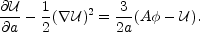
Munshi and Starobinsky (1994) point out that the standard Zel'dovich approximation is equivalent to the assumption that = phi t, while the Frozen Flow approximation is = phi ₀ t and the Frozen (or Linear) Potential approximation is Phi = phi ₀. In any case, this last equation provides an equation for the velocity potential given a model for the gravitational potential.

More recently, we have seen the "Truncated" Zel'dovich Approximation (Coles et al., 1993; Melott et al., 1994b), the "Optimized" Zel'dovich Approximation (Melott et al., 1994c) and the "Completed" Zel'dovich Approximation (Betancort-Rijo and López-Corredoira, 2000). These correlate remarkably well with full N-body simulations.

5. Nonlinear enhancements

Various authors have presented nonlinear versions of the Zel'dovich approximation. Gramann (1993); Susperregi and Buchert (1997) used a second order extension, while Buchert (1994) presented a perturbation scheme that is correct to third order in small quantities.