B.4.9. Stellar Dynamics and Lensing

Stellar dynamical analyses of gravitational lenses have reached the level of studies of local galaxies approximately 15-20 years ago. The analyses are based on the spherical Jeans equations (see Binney & Tremaine [1987]) with simple models of the orbital anisotropy and generally ignore both deviations from sphericity and higher order moments of the velocity distributions. The spherical Jeans equation

(B.90)

relates the radial velocity dispersion _r = <v_r²>^1/2, the isotropy parameter (r) = 1 - ² / _r² characterizing the ratio of the tangential dispersion to the radial dispersion, the luminosity density of the stars (r) and the mass distribution M(r). A well known result from dynamics is that you cannot infer the mass distribution M(r) without constraining the isotropy (r) (e.g. Binney & Mamon [1982]). Models with = 0 are called isotropic models (i.e. _r = ), while models with 1 are dominated by radial orbits ( 0) and models with - are dominated by tangential orbits ( _r 0) . These 3D components of the velocity dispersion must then be projected to measure the line-of-sight velocity dispersion <v_los²>^1/2,

(B.91)

where (R) = 2₀ dz(r) is the projected surface brightness and z is the coordinate along the line of sight.

Modern observations of local galaxies break the degeneracy between mass and isotropy by measuring higher order moments (<v_losⁿ>) of the line-of-sight velocity distribution (LOSVD) because the shape of the LOSVD is affected by the isotropy of the orbits. Because the velocity dispersions are measured starting from a Gaussian fit to the LOSVD, the higher order moments are described by the amplitudes h_n of a decomposition of the LOSVD into Gauss-Hermite polynomials (e.g. van der Marel & Franx [1993]). In general, the rms velocity (i.e. combining dispersion and rotation) and higher order moment profiles of early-type galaxies are fairly self-similar, with nearly flat rms velocity profiles, modest values of h₄ 0.01 ± 0.03 and slightly radial orbits <> 0.1-0.2 (e.g. Romanowsky & Kochanek [1999], Gerhard et al. [2001]).

Stellar dynamics is used for two purposes in lensing studies. The first is to provide a mass normalization for lens models used in studies of lens statistics. We will discuss this in Section B.6. The second is to use comparisons between a mass estimated from the geometry of a lens and the velocity dispersion of the lens galaxy to constrain the mass distribution (e.g. Romanowsky & Kochanek [1999], Trott & Webster [2002], Koopmans & Treu [2002], [2003], Treu & Koopmans [2002a], [2002b], Koopmans et al. [2003]). It is important to understand that the systematic uncertainties in combining lensing and stellar dynamics to determine mass distributions are different from using either in isolation. For local galaxies we measure a velocity dispersion profile. The normalization of the profile sets the mass scale and the changes in the profile (and any higher order moments) with radius constrains the mass distribution. To lowest order, a simple scaling error in the velocity measurements will lead to errors in the mass scale rather than in the mass distribution. For lens galaxies, it is the comparison between the velocity dispersion and the mass determined by the geometry of the images that constrains the mass distribution. Thus, estimates of the mass distribution are directly affected by any calibration errors in the velocity dispersions.

We can understand the differences with a simple thought experiment. Suppose we have a mass distribution M = M₀(R / R₀)^x in projection and we have mass estimates M₁ at R₁ and M₂ at R₂. Combining them we can solve for the exponent describing the mass distribution, x = ln(M₁/M₂) / ln(R₁ / R₂). In a dynamical observation the mass estimate is some sort of virial estimator M _v² R / G while in a lensing measurement it is a direct measurement of M. Standard velocity dispersion measurements start from the best fit Gaussian line width and then subtract an intrinsic line width _c due to the instrument and the intrinsic line width of the star in quadrature to estimate the portion of the line width due to the motions of the stars. Thus _v² = f²(² - _c²) where f 1 is a scale factor to account for deviations from spherical symmetry and non-Gaussian line of sight velocity distributions (LOSVDs). In a purely dynamical study, uncertainties in f and _c produce bigger fractional errors in the absolute mass scale M₀ than in the exponent x. For example, given measurements ₁ and ₂ at radii R₁ and R₂, the exponent, x = 1 + ln(₁² /₂²) / ln(R₁ / R₂), depends only on velocity dispersion ratios in which calibration errors tend to cancel. This is obvious for the scale factor f, which cancels exactly if it does not vary with radius. Since studies of lens dynamics use a comparison between a dynamical mass and a lensing mass to estimate the mass distribution, the results are more sensitive to calibration problems because these cancellations no longer occur. If we combine a velocity dispersion measurement ₁ with a lensing mass measurement M₂ our estimate of the exponent becomes x = ln(₁² R₁ / GM₂) / ln(R₁ / R₂) and the uncertainties are linear in the scale factor f rather than canceling. An error analysis for the effects of _c is messier, but you again find that the sensitivity in the mixed lensing and dynamics constraint to errors in _c is greater than in a purely dynamical study.

Velocity dispersions have now been measured for 10 lenses (0047-2808 Koopmans & Treu [2003]; CFRS03.1077 Treu & Koopmans [2004]; Q0957+561 Falco et al. [1997], Tonry & Franx [1999]; PG1115+080 Tonry [1998]); HST14176+5226 Ohyama et al. [2002], Gebhardt et al. [2003], Treu & Koopmans [2004]; HST15433+5352 Treu & Koopmans [2004]; MG1549+3047 Lehár et al. [1996]; B1608+656 Koopmans et al. [2003]; MG2016+112 Koopmans & Treu [2002]; Q2237+0305 Foltz et al. [1992]). With the exception of Romanowsky & Kochanek ([1999]), who fitted for the distribution function of the lens, the analyses of the data have used the spherical Jeans equations with parameterized models for the isotropy (r). They include the uncertainties in _c about as well as any other dynamical study, although it is worth bearing in mind that this is tricky because we lack nearby stars with the appropriate metallicity and the problem of matching the spectral resolution for the galaxy and the template stars lacks direct checks of the success of the procedure. A useful rule of thumb to remember is that repeat measurements of velocity dispersions by different groups almost always show larger scatter than is consistent with the reported uncertainties. For example, the three velocity dispersion measurements for the lens HST14176+5226 (224 ± 15 km/s by Ohyama et al. [2002], 202 ± 9 km/s by Gebhardt et al. [2003], and 230 ± 14 km/s by Treu & Koopmans [2004]) are mutually consistent only if the uncertainties are broadened by 30%.

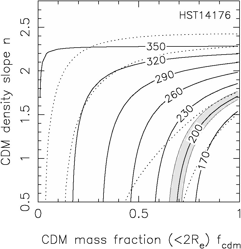
In Fig. B.33 we summarize the dynamical constraints for 9 of these systems using the self-similar mass distribution from Rusin & Kochanek ([2004], Eqn. B.89). This model is very similar to that used by Treu & Koopmans ([2004]). For most of the lenses, the region producing a good fit to the combined lensing and dynamical data overlaps the same region preferred by the Rusin & Kochanek ([2004]) self-similar models, shows the same general parameter degeneracy and is consistent with a simple SIS mass distribution (f_cdm 1 and n = 2). This is particularly true of 0047-2808, HST15433+5352, B1608+656, MG2016+112 and CFRS03.1077. Only Q2237+0305, where the lens is the bulge of a nearby spiral and we might not expect this mass model to be applicable, shows a very different trend (e.g. see the models of Trott & Webster [2002]). PG1115+080 and to a lesser extent MG1549+3047 might have steeper than isothermal mass distributions (falling rotation curves) and the possibility of being consistent with a constant mass-to-light ratio model (Treu & Koopmans [2002a]). HST14176+5226 and to a lesser extent HST15433+5352 could have shallower than isothermal mass distribution (rising rotation curves). Along the degeneracy direction for each lens we will find similar mass distributions with very different decompositions into luminous and dark matter, just as in Fig. B.32. The problem raised by this panorama is whether it shows that the halo structure is largely homogeneous with some measurement outliers, or that the structure of early-type is heterogeneous with important implications for understanding time delays (Section B.5) and galaxy evolution (Section B.9).

Figure B.33. Constraints from lens velocity dispersion measurements on the self-similar mass distributions of Eqn.B.89 and Fig. B.32. The dotted contours show the 68% and 95% confidence limits from the self-similar models for Rb / Re = 50. The shaded regions show the models allowed (68% confidence) by the formal velocity dispersion measurement errors, and the heavy solid lines show contours of the velocity dispersion in km/s. We used the low Gebhardt et al. ([2003]) velocity dispersion for HST14176+5226 because it has the smallest formal error. These models assumed isotropic orbits, thereby underestimating the full uncertainties in the stellar dynamical models.

My own view tends toward the first interpretation - that the dynamical data supports the homogeneity of early-type galaxy structure. The permitted bands in Fig. B.33 show the 68% confidence regions given the formal measurement errors and the simple, spherical, isotropic Jeans equation models - this means that the true 68% confidence regions are significantly larger. We have already argued that the formal errors on dynamical measurements tend to be underestimates. For example, the need for HST14176+5226 to have a rising rotation curve would be considerably reduced if we used the higher velocity dispersion measurements from Ohyama et al. ([2002]) or Treu & Koopmans ([2004]) or if we broadened the uncertainties by the 30% needed to make the three estimates statistically consistent. Moreover, the existing analyses have also neglected the systematic uncertainties arising from the scaling factor f. There are two important issues that make f 1. The first issue is that standard velocity dispersion measurements are the width of the best fit Gaussian model for the LOSVD, and this is not the same as the mean square velocity (<v_los²>^1/2) appearing in the Jeans equations used to analyze the data unless the LOSVD is also a Gaussian. Stellar dynamics has adopted the dimensionless coefficients h_n of a Gauss-Hermite polynomial series to model the deviations of the LOSVD from Gaussian, and a typical early-type galaxy has | h₄| 0.03 (e.g. Romanowsky & Kochanek [1999]). This leads to a systematic difference between the measured dispersions and the mean square velocity of <v_los²>^1/2 (1 + 6^1/2 h₄) (e.g. van der Marel & Franx [1993])), so | f - 1| ~ 7% for | h₄| 0.03. Only the Romanowsky & Kochanek [1999]) models of Q0957+561 and PG1115+080 have properly included this uncertainty. In fact, Romanowsky & Kochanek ([1999]) demonstrated that there were stellar distribution functions in which the mass distribution of PG1115+080 is both isothermal and agrees with the measured velocity dispersion. While it is debatable whether these models allowed too much freedom, it is certainly true that models using the Jeans equations and ignoring the LOSVD have too little freedom and will overestimate the constraints.

The second issue is that lens galaxies are not spheres. Unfortunately there are few simple analytic results for oblate or triaxial systems like early-type galaxies in which the ellipticity is largely due to anisotropies in the velocity dispersion tensor rather than rotation. For the system as a whole, the tensor virial theorem provides a simple global relationship between the major and minor axis velocity dispersions

(B.92)

for an oblate ellipsoid of axis ratio q and eccentricity e = (1 - q²)^1/2 (e.g. Binney & Tremaine [1987]). The velocity dispersion viewed along the major axis is larger than that on the minor, and the correction can be quite large since a typical galaxy with q = 0.7 will have a ratio _major / _minor 1.16 that is much larger than typical measurement uncertainties. If galaxies are oblate, this provides no help for the case of PG1115+080 because making the line-of-sight dispersion too high requires a prolate galaxy. However, it is a very simple means of shifting HST14176+5226. Crudely, if we start with the low 209 km/s velocity dispersion and assume that the lens is an q = 0.7 galaxy viewed pole on, then _major / _minor 1.14 and the corrections for the shape are large enough to make HST14176+5226 consistent with the other systems.

A final caveat is that neglecting necessary degrees of freedom in your lens model can bias inferences from the stellar dynamics of lenses just as it can in pure lens modeling. For example, Sand et al. ([2002], [2003]) used a comparison of lensed arcs in clusters to velocity dispersion measurements of the central cluster galaxy to argue that the cluster dark matter distribution could not have the 1 / r cusp of the NFW model for CDM halos. However, Bartelmann & Meneghetti ([2003]) and Dalal & Keeton ([2003]) show that the data are consistent with an NFW cusp if the lens models include a proper treatment of the non-spherical nature of the clusters. This has not been an issue in the stellar dynamics of strong lenses where the lens models used to determine the mass scale have always included the effects of ellipticity and shear, but it is well worth remembering.