B.5.1. A General Theory of Time Delays

Just as for estimating mass distributions (Section B.4), the aspect of modeling time delays that creates the greatest suspicion is the need to model the gravitational potential of the lens. Just as for mass distributions, this problem is largely of our own making, arising from poor communication, understanding and competition between groups. Here we will use simple mathematical expansions to show exactly what properties of the potential determine time delays. Any models which have these generic properties have all the degrees of freedom needed to properly interpret time delays. This does not, unfortunately, avoid the problem of degeneracies between the mass models and the Hubble constant.

The key to understanding time delays comes from Gorenstein, Falco & Shapiro ([1988], Kochanek [2002a], see also Saha [2000]) who showed that the time delay in a circular lens depends only on the image positions and the surface density () in the annulus between the images. The two lensed images at radii _A > _B define an annulus bounded by their radii, with an interior region for < _B and an exterior region for > _A (Fig. B.20). As we discussed in Section B.4.1, the mass in the interior region is implicit in the image positions and constrained by the astrometry. From Gauss' law we know that the distribution of the mass in the interior and the amount or distribution of mass in the exterior region is irrelevant (see Section B.4.3). A useful approximation is to assume that the surface density in the annulus can be locally approximated by a power law, () ^1-n for _B < < _A, with a mean surface density in the annulus of <> = <> / _c. The time delay between the images is then (Kochanek [2002a])

(B.97)

where <> = (_A + _B) / 2 and = _A - _B as before. Thus, the time delay is largely determined by the average surface density <> in the annulus with only modest corrections from the local shape of the surface density distribution even when / <> ~ 1. This second order expansion is exact for an SIS lens (<> = 1/2, n = 2), and it reproduces the time delay of a point mass lens (<> = 0) to better than 1% even when / <> = 1. The local model also explains the scalings of the global power-law models. A ^1-n global power law has surface density <> = (3 - n) / 2 near the Einstein ring, so the leading term of the time delay is t = 2_SIS(1 - <>) = (n - 1)t_SIS just as in Eqn. B.96.

The role of the angular structure of the lens is easily incorporated into the expansion through the multipole expansion of Section B.4. A quadrupole term in the potential with dimensionless amplitude produces ray deflections of order O(b) at the Einstein radius b of the lens. In a four-image lens, the quadrupole deflections are comparable to the fractional thickness of the annulus, / <>, while in a two-image lens they are smaller. For an ellipsoidal density distribution, the cos(2m) multipole amplitude is smaller than the quadrupole amplitude by _2m ~ ^m ( / <>)^m. Hence, to lowest order in the expansion we only need to include the internal and external quadrupoles of the potential but not the changes of the quadrupoles in the annulus or any higher order multipoles. Remember that what counts is the angular structure of the potential rather than of the density, and that potentials are always much rounder than densities with a typical scaling of m^-2:m^-1:1 between the potential, deflections and surface density for the cos m multipoles (see Section B.4.4)

While the full expansion for independent internal and external quadrupoles is too complex to be informative, the leading term for the case when the internal and external quadrupoles are aligned is informative. We have an internal shear of amplitude and an external shear of amplitude with = as defined in Eqns. B.51 and B.52. The leading term of the time delay is

(B.98)

where _AB is the angle between the images (Fig. B.20) and f_int = / ( + ) is the internal quadrupole fraction we explored in Fig. B.31. We need not worry about a singular denominator - successful models of the image positions do not allow such configurations.

A two-image lens has too few astrometric constraints to fully constrain a model with independent, misaligned internal and external quadrupoles. Fortunately, when the lensed images lie on opposite sides of the lens galaxy ( _AB + with || << 1), the time delay becomes insensitive to the quadrupole structure. Provided the angular deflections are smaller than the radial deflections (|| <> ), the leading term of the time delay reduces to the result for a circular lens, t = 2t_SIS(1 - <>) if we minimize the total shear of the lens. In the minimum shear solution the shear converges to the invariant shear (₁) and the other shear component ₂ = 0 (see Section B.4.5). If, however, you allow the other shear component to be non-zero, then you find that t = 2t_SIS(1 - <> - ₂) to lowest order - the second shear component acts like a contribution to the convergence. In the absence of any other constraints, this adds a modest additional uncertainty (5-10%) to interpretations of time delays in two-image lenses. To first order its effects should average out in an ensemble of lenses because the extra shear has no preferred sign.

A four image lens has more astrometric constraints and can constrain a model with independent, misaligned internal and external quadrupoles - this was the basis of the Turner et al. ([2004]) summary of the internal to total quadrupole ratios shown in Fig. B.31. If the external shear dominates, then f_int 0 and the leading term of the delay becomes t = 2 t_SIS(1 - <>)sin² _AB / 2. If the model is isothermal, like the = F() model we introduced in Eqn. B.42, then f_int = 1/4 and we obtain the Witt et al. ([2000]) result that the time delay is independent of the angle between the images t 2 t_SIS(1 - <>). Thus, delay ratios in a four-image lens are largely determined by the angular structure and provide a check on the potential model. Unfortunately, the only lens with precisely measured delay ratios, B1608+656 (Fassnacht et al. [2002]), also has two galaxies inside the Einstein ring and is a poor candidate for a simple multipole treatment (although it is dominated by an internal quadrupole as expected, see Fig. B.31). The delay ratios for PG1115+080 are less well measured (Schechter et al. 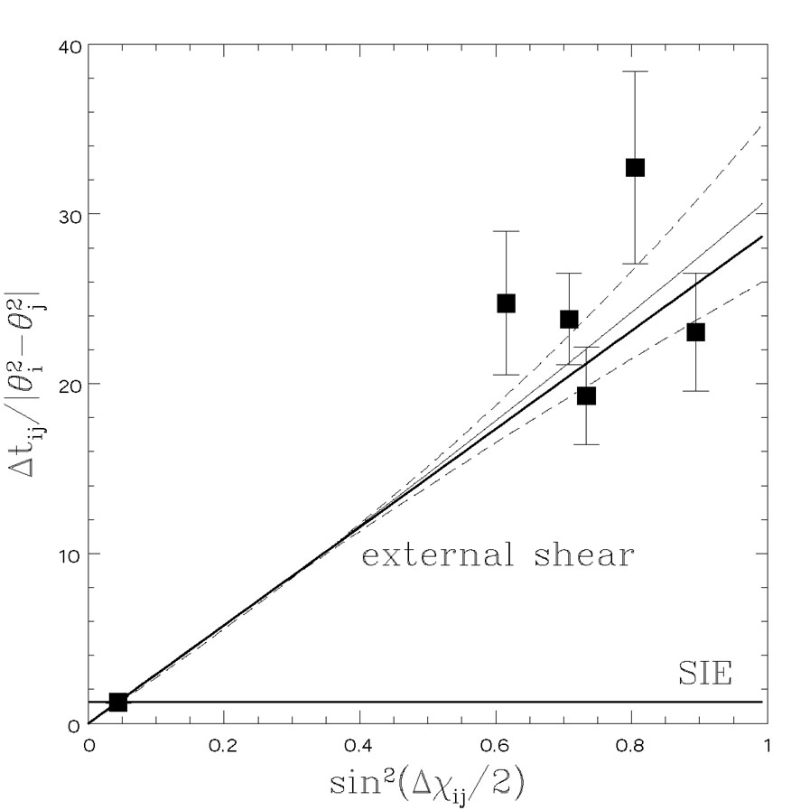[1997], Barkana [1997], Chartas [2003]), but should be dominated by external shear since the estimate from the image astrometry is that f_int = 0.083 (0.055 < f_int < 0.111 at 95% confidence). Fig. B.34 shows the dependence of the PG1115+080 delays on the leading angular dependence of the time delay (Eqn. B.98) after scaling out the standard astrometry factor for the different radii of the images (Eqn. B.94). Formally, the estimate from the time delays that f_int = - 0.02 (-0.09 < f_int < 0.03 at 68% confidence) is a little discrepant, but the two estimates agree at the 95% confidence level and there are still some systematic uncertainties in the shorter optical delays of PG1115+080. Changes in f_int between lenses is the reason Saha ([2004]) found significant scatter between time delays scaled only by t_SIS, since the time delay lenses range from external shear dominated systems like PG1115+080 to internal shear dominated systems like B1608+656.

Figure B.34. (Top) The PG1115+080 time delays scaled by the astrometric factor i2 - j2 appearing in tSIS (Eqn. B.94) as a function of the leading angular dependence of the time delay (sin2 ij / 2) (Eqn. B.98). The light solid curve and the dashed curves show the dependence for the best fit internal shear fraction fint and its 68% confidence limits. A true external shear fint = 0 is shown by the heavy solid curve inside the confidence limits, and the scaling for an SIE ( fint = 1/4) is shown by the horizontal line. (Bottom) The 2 goodness of fit for the internal shear fraction fint from the time delay ratios is shown by the curve with the 68% confidence region bracketed by the vertical lines. The estimate of fint from the image astrometry is shown by the point with an error bar.