K. Orphan Afterglows

Orphan afterglows arise as a natural prediction of GRB jets. The realization that GRBs are collimated with rather narrow opening angles, while the following afterglow could be observed over a wider angular range, led immediately to the search for orphan afterglows: afterglows which are not associated with observed prompt GRB emission. While the GRB and the early afterglow are collimated to within the original opening angle, _j, the afterglow can be observed, after the jet break, from a viewing angle of ^-1. The Lorentz factor, , is a rapidly decreasing function of time. This means that an observer at _obs > _j couldn't see the burst but could detect an afterglow once ^-1 = _obs. As the typical emission frequency and the flux decrease with time, while the jet opening angle increases, this implies that observers at larger viewing angles will detect weaker and softer afterglows. X-ray orphan afterglows can be observed several hours or at most a few days after the burst (depending of course on the sensitivity of the detector). Optical afterglows (brighter than 25th mag ) can be detected in R band for a week from small (~ 10°) angles away from the GRB jet axis. On the other hand, at very late times, after the Newtonian break, radio afterglows could be detected by observers at all viewing angles.

The search for orphan afterglows is an observational challenge. One has to search for a 10^-12 ergs/sec/cm² signal in the X-ray, a 23th or higher magnitude in the optical or a mJy in radio (at GHz) transients. Unlike afterglow searches that are triggered by a well located GRB for the orphan afterglow itself there is no information where to search and confusion with other transients is rather easy. So far there was no detection of any orphan afterglow in any wavelength.

Rhoads [343] was the first to suggest that observations of orphan afterglows would enable us to estimate the opening angles and the true rate of GRBs. Dalal et al. [69] have pointed out that as the post jet-break afterglow light curves decay quickly, most orphan afterglows will be dim and hence undetectable. They point out that if the maximal observing angle, _max, of an orphan afterglow will be a constant factor times _j the ratio of observed orphan afterglows, R_orph^obs, to that of GRBs, R_GRB^obs, will not tell us much about the opening angles of GRBs and the true rate of GRBs, R_GRB^true f_b R_GRB^obs. However as we see below this assumption is inconsistent with the constant energy of GRBs that suggests that all GRBs will be detected to up to a fixed angle which is independent of their jet opening angle.

1. Optical Orphan Afterglow

Optical orphan afterglow is emitted at a stage when the outflow is still relativistic. The observation that GRBs have a roughly constant total energy [105, 291, 310] and that the observed variability in the apparent luminosity arises mostly from variation in the jet opening angles leads to a remarkable result: The post jet-break afterglow light curve is universal [139]. Fig. 31 depicts this universal light curve. This implies that for a given redshift, z, and a given limiting magnitude, m, there will be a fixed _max(z, m) (independent of _j, for _j < _max) from within which orphan afterglow can be detected.

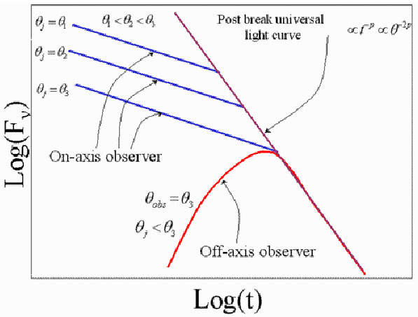Figure 31. A schematic afterglow light curve. While the burst differ before the jet break (due to different opening angles, the light curve coincide after the break when the energy per unit solid angle is a constant.

This universal post jet-break light curve can be estimated from the observations [409] or alternatively from first principles [273] . An observer at _obs > _j will (practically) observe the afterglow emission only at t when = _obs^-1. Using Eq. 104 and the fact that t^-1/2 after the jet break (Eq. 106) one can estimate the time, t when a emission from a jet would be detected at _obs:

(109)

where A is a factor of order unity, and t_jet is the time of the jet break (given by Eq. 104). The flux at this time is estimated by substitution of this value into the post-jet-break light curve (see Nakar et al. [273] for details):

(110)

where F₀ is a constant and f (z) = (1 + z)¹⁺ D_L28^-2 includes all the cosmological effects and D_L28 is the luminosity distance in units of 10²⁸ cm. One notices here a very strong dependence on _obs. The peak flux drops quickly when the observer moves away from the axis. Note also that this maximal flux is independent of the opening angle of the jet, _j. The observations of the afterglows with a clear jet break (GRB 990510 [159, 394], and GRB 000926 [160]) can be used to calibrate F₀.

Now, using Eq. 110, one can estimate _max(z, m) and more generally the time, (t_obs(z, , m) that a burst at a redshift, z, can be seen from an angle above a limiting magnitude, m:

(111)

One can then proceed and integrate over the cosmological distribution of bursts (assuming that this follows the star formation rate) and obtain an estimate of the number of orphan afterglows that would appear in a single snapshot of a given survey with a limiting sensitivity F_lim:

(112)

where n(z) is the rate of GRBs per unit volume and unit proper time and dV(z) is the differential volume element at redshift z. Note that modifications of this simple model may arise with more refined models of the jet propagation [139, 273].

The results of the intergration of Eq. 112 are depicted in Fig. 32. Clearly the rate of a single detection with a given limiting magnitude increases with a larger magnitude. However, one should ask what will be the optimal strategy for a given observational facility: short and shallow exposures that cover a larger solid angle or long and deep ones over a smaller area. The exposure time that is required in order to reach a given limiting flux, F_lim, is proportional to F_lim^-2. Dividing the number density of observed orphan afterglows (shown in Fig. 32) by this time factor results in the rate per square degree per hour of observational facility. This rate increases for a shallow surveys that cover a large area. This result can be understood as follows. Multiplying Eq. 112 by F_lim² shows that the rate per square degree per hour of observational facility F_lim^2-2/p. For p > 1 the exponent is positive and a shallow survey is preferred. The limiting magnitude should not be, however, lower than ~ 23rd as in this case more transients from on-axis GRBs will be discovered than orphan afterglows.

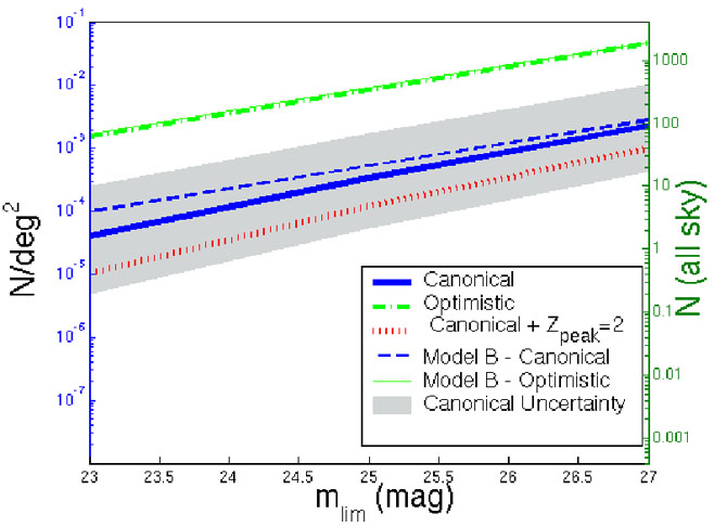Figure 32. The number of observed orphan afterglows per square degree (left vertical scale) and in the entire sky (right vertical scale), in a single exposure, as a function of the limiting magnitude for detection. The thick lines are for model A with three different sets of parameters: i) Our "canonical" normalization F0 = 0.003 µJy, zpeak = 1, j = 0.1 (solid line). The gray area around this line corresponds an uncertainty by a factor of 5 in this normalization. ii) Our most optimistic model with a relatively small j = 0.05 and a large F0 = 0.015 µJy (dashed-dotted line). iii) The same as our "canonical" model, except for zpeak = 2 (dotted line). The thin lines are for model B, where the solid line is for our "optimistic" parameters, while the dashed line is for our "canonical" parameters. Both models are similar for the "optimistic" parameters while model B predicts slightly more orphan afterglows then model A for the "canonical" parameters. From [273]

Using these estimates Nakar et al. [273] find that with their most optimistic parameters 15 orphan afterglows will be recorded in the Sloan Digital Sky Survey (SDSS) (that covers 10⁴ square degrees at 23rd mag) and 35 transients will be recorded in a dedicated 2m class telescope operating full time for a year in an orphan afterglow search. Totani and Panaitescu [409] find a somewhat higher rate (a factor ~ 10 above the optimistic rate). About 15% of the transients could be discovered with a second exposure of the same area provided that it follows after 3, 4 and 8 days for m_lim = 23, 25 and 27. This estimate does not tackle the challenging problem of identifying the afterglows within the collected data. Rhoads [345] suggested to identify afterglow candidates by comparing the multi-color SDSS data to an afterglow template. One orphan afterglow candidate was indeed identified using this technique [420]. However, it turned out that it has been a variable AGN [118]. This event demonstrates the remarkable observational challenge involved in this project.

2. Radio Orphan Afterglow

After the Newtonian transition the afterglow is expanding spherical. The velocities are at most mildly relativistic so there are no relativistic beaming effects and the afterglow will be observed from all viewing angles. This implies that observations of the rate of orphan GRB afterglows at this stage will give a direct measure of the beaming factor of GRBs. Upper limits on the rate of orphan afterglows will provide a limit on the beaming of GRBs [298]. However, as I discuss shortly, somewhat surprisingly, upper limits on the rate of orphan radio afterglow (no detection of orphan radio afterglow) provide a lower (and not upper) limit on GRB beaming [215].

Frail et al. [107] estimate the radio emission at this stage using the Sedov-Taylor solution for the hydrodynamics (see Section VIID). They find that the radio emission at GHz will be around 1 mJy at the time of the Newtonian transition (typically three month after the burst) and it will decrease like t^{-3(p-1)/2+3/5} (see Eq. 97). Using this limit one can estimate the rate of observed orphan radio afterglow within a given limiting flux. The beaming factor f^-1_b arises in two places in this calculations. First, the overall rate of GRBs: R_GRB^true f_b R_GRB^obs, increases with f_b. Second the total energy is proportional to f_b^-1 hence the flux will decrease when f_B increases. The first factor implies that the rate of orphan radio afterglows will increase like f_b. To estimate the effect of the second factor Levinson et al. [215] use the fact that (for a fixed observed energy) the time that a radio afterglow is above a given flux is proportional to E^10/9 in units of the NR transition time which itself is proportional to E^1/3. Overall this is proportional to E^13/9 and hence to f_b^-13/9. To obtain the overall effect of f_b Levinson et al. [215] integrate over the redshift distribution and obtain the total number of orphan radio afterglow as a function of f_b. For a simple limit of a shallow survey (which is applicable to current surveys) typical distances are rather "small", i.e. less than 1 Gpc and cosmological corrections can be neglected. In this case it is straight forwards to carry the integration analytically and obtain the number of radio orphan afterglows in the sky at any given moment [215]:

(113)

where R is the observed rate of GRBs per Gpc³ per year, and t_i is the time in which the radio afterglow becomes isotropic.

Levinson et al. [215] search the FIRST and NVSS surveys for point-like radio transients with flux densities greater than 6 mJy. They find 9 orphan candidates. However, they argue that the possibility that most of these candidates are radio loud AGNs cannot be ruled out without further observations. This analysis sets an upper limit for the all sky number of radio orphans, which corresponds to a lower limit f_b^-1 > 10 on the beaming factor. Rejection of all candidates found in this search would imply f_b^-1 > 40 [153].