7.3. Angular Variability and Other Caveats

In a Type-I model, that is a for a shell satisfying < R_E / _E², variability is possible only if the emitting regions are significantly narrower than _E^-1. The source would emit for a total duration T_radial. To estimate the allowed opening angle of the emitting region imagine two points that emit radiation at the same (observer) time t. The difference in the arrival time between two photons emitted at (R_E, ₁) and (R_E, ₂) at the same (observer) time t is:

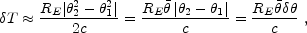(35)

where is the angle from the line of sight and we have used ₁, ₂ << 1, (₁ + ₂) / 2 and |₂ - ₁|. Since an observer sees emitting regions up to an angle _E^-1 away from the line of sight ~ _E^-1. The size of the emitting region r_s = R_E is limited by:

(36)

The corresponding angular size is:

(37)

Note that Fenimore, Madras and Nayakshin [230] who examined this issue, considered only emitting regions that are directly on the line of sight with ~ |₂ - ₁| and obtained a larger r_s which was proportional to R_E^1/2. However only a small fraction of the emitting regions will be exactly on the line of sight. Most of the emitting regions will have ~ _E^-1, and thus Eq. 36 yields the relevant estimate.

The above discussion suggests that one can produce GRBs with T T_radial R_E / c_E² and T = T / if the emitting regions have angular size smaller than 1 / _E 10^-4. That is, one needs an extremely narrow jet. Relativistic jets are observed in AGNs and even in some galactic objects, however, their opening angles are of order of a few degrees almost two orders of magnitude larger. A narrow jet with such a small opening angle would be able to produce the observed variability. Such a jet must be extremely cold (in its local rest frame); otherwise its internal pressure will cause it to spread. It is not clear what could produce such a jet. Additionally, for the temporal variability to be produced, either a rapid modulation of the jet or inhomogeneities in the ISM are needed. These two options are presented in Fig. 16.

Figure 16. A very narrow jet of angular size considerably smaller than e-1, for which the angular spreading problem does not exist. The duration of the burst is determined by the deceleration distance Re, while the angular time is assumed small. The variability could now be explained by either variability in the source which leads to a pulsed jet (a) or by a uniform jet interacting with an irregular ISM (b)

A second possibility is that the shell is relatively "wide" (wider than _E^-1) but the emitting regions are small. An example of this situation is schematically described in Fig. 17. This may occur if either the ISM or the shell itself are very irregular. This situation is, however, extremely inefficient. The area of the observed part of the shell is R_E² / _E². The emitting regions are much smaller and to comply with the temporal constraint their area is r_s². For high efficiency all the area of the shell must eventually radiate. The number of emitting regions needed to cover the shell is at least (R_E / _E r_s)². In Type-I models, the relation R_E = 2c _E² T holds, and the number of emitting region required is 4². But a sum of 4² peaks each of width 1 / of the total duration does not produce a complex time structure. Instead it produces a smooth time profile with small variations, of order 1 / (2 )^1/2 << 1, in the amplitude.

Figure 17. A shell with angular size -1 (the angular size is highly exaggerated). The spherical symmetry is broken by the presence of bubbles in the ISM. The relative angular size of the shell and the bubbles is drawn to scale assuming that a burst with N = 15 is to be produced. Consequently N = 15 bubbles are drawn (more bubbles will add up to a smooth profile). The fraction of the shell that will impact these bubbles is small leading to high inefficiency. As N increases the efficiency problem becomes more severe ~ N-1, from [20]

In a highly variable burst there cannot be more than sub-bursts of duration T = T / . The corresponding area covering factor (the fraction of radiating area of the shell) and the corresponding efficiency is less than 1 / 4. This result is independent of the nature of the emitting regions: ISM clouds, star light or fragments of the shell. This is the case, for example, in the Shaviv & Dar model [235] where a relativistic iron shell interacts with the starlight of a stellar cluster (a spherical shell interacting with an external fragmented medium). This low efficiency poses a series energy crisis for most (if not all) cosmological models of this kind. In a recent paper Fenimore et al. [231] consider other ways, which are based on low surface covering factor, to resolve the angular spreading problems. None seems very promising.