2. THE LUMINOSITY FUNCTION OF FIELD GALAXIES

The luminosity function (M_R), is defined such that (M_R) dM_R is the number of galaxies in the absolute R-band magnitude range [M_R, M_R + dM_R] ⁴. The field galaxy luminosity function is plotted by Hubble Type in figure 1. As in [Trentham et al. 2005], the bright end of the luminosity function was computed using data from the SDSS galaxy survey, while the faint end was taken from observations of nearby galaxy groups (e.g. [Trentham & Tully 2002]). We show parameter values on the plot for a Schechter function fit to the luminosity function ⁵. While the error bars are small enough that the Schechter function does not provide a good formal fit, it is a simple analytic form which captures the main features of the mass and luminosity functions which are presented in this paper.

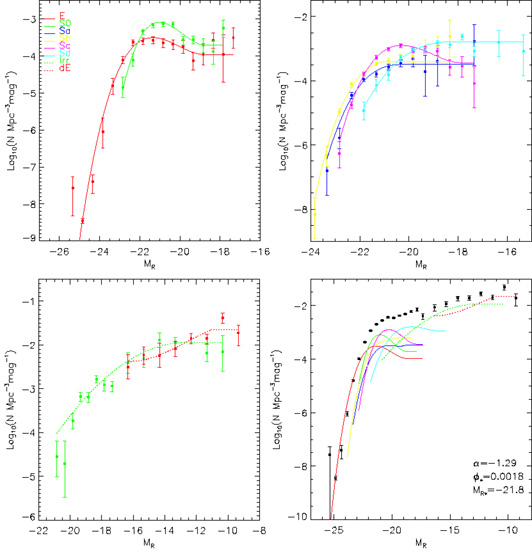Figure 1. The field galaxy luminosity function split by Hubble Type. The top left plot is for Elliptical and S0 galaxies, the top right is for spirals (Sa-Sd), the bottom left is for the dwarf galaxies (irregular and elliptical) and the bottom right is the combined luminosity function. In each plot a spline-fit to the luminosity function is shown to guide the eye and these spline fits are also overlaid on the combined luminosity function in the bottom right plot. Galaxies which are very luminous in the R-band lie to left of these plots, while those which are very faint lie to the right. Overlaid on the bottom right panel are parameters for a Schechter fit to the total luminosity function.

The Hubble Type is a subjective assessment that depends on many parameters that can be measured for nearby bright galaxies. It cannot be determined for the faint galaxies in SDSS images, so we cannot determine type-specific luminosity functions from SDSS data alone. Broadband colours are often regarded as a straightforward way to distinguish between different kinds of galaxies. These are available for the SDSS sample, but this is a poor discriminant since different Hubble Types can have very similar colours ([Fukugita et al. 1995]), particularly different kinds of spiral galaxies. Another discriminant is the light concentration parameter, but this alone cannot be used to distinguish different types of late-type galaxies: concentration parameters do not depend on scale length if the profiles are exponential. H emission-line strength is yet another discriminant, but there is considerable scatter in the H equivalent width of galaxies of a single Hubble type ([Kennicutt & Kent 1983]).

We therefore, use the following procedure. Brightward of M_R = - 17.5, concentration parameters, K-corrected ⁶ broadband colours, and H equivalent widths were used in conjunction with each other to classify the SDSS galaxies as early-type, intermediate-type, or late-type using local galaxies as templates. Luminosity functions were computed for each. The early-type luminosity function was then further split into an elliptical luminosity function and an S0 luminosity function in such a way that the relative numbers of these kinds of galaxies corresponded to that in each magnitude range in the Nearby Galaxies Catalogue ([Tully 1988]), which lists a sample of luminous galaxies within 40 Mpc. The intermediate luminosity function was split into an Sa luminosity function and an Sb luminosity function similarly. The late-type luminosity function was split into an Sc, an Sd, and an irregular luminosity function. Brightward of M_R = - 17.5, dwarf elliptical galaxies do not seem to exist outside rich clusters (see e.g. [Binggeli et al. 1988]). Faintward of M_R = - 17.5, the luminosity function was split according to the relative numbers of the different kinds of galaxies in the groups surveyed by [Trentham & Tully (2002)] and the Local Group.

This method of computing the luminosity function is motivated by our need to obtain stellar mass-to-light ratios and gas masses or galaxies of particular magnitudes and types. It forces the SDSS galaxy sample to have properties similar to the local galaxy sample, but it generates a luminosity function that is less susceptible to cosmic variance problems than a luminosity function derived from the local galaxy sample alone. Our method is subject to systematic problems if the two galaxy samples are very different. Other authors have used concentration parameters (see e.g. [Kauffmann et al. 2003]) or star formation histories derived from the SDSS spectra ([Panter et al. 2004]) to determine the mass-to-light ratios. Comparing our results to other values in the literature will be an important test of our method.

A comparison between our luminosity function and one derived from measurements of local galaxies alone ([Binggeli et al. 1988]) is also interesting. The main difference is that we find many more late-type star-forming galaxies at low and intermediate luminosities. This is perhaps to be expected given the very steep rise of the ultraviolet luminosity density and star-formation rate of the Universe with redshift ( I (1 + z)³; [Giavalisco et al. 2004] [Giavalisco et al. 2004]), which would lead us to expect about twice times as many star-forming galaxies per luminous early-type galaxy at z ~ 0.1 (the typical redshift of the SDSS galaxies) than at z = 0.

⁴ The absolute magnitude is a logarithmic measure of the luminosity in the R-band. Historically, the luminosity of galaxies is presented as M_X = - 2.5 log_{10 X} L T_X() d + constant where X denotes some filter (e.g. R-band), T_X() is the transmission function of that filter, and L is the spectral energy distribution of the galaxy. The nomenclature for filters is complicated because many groups define their own system. Often these labels overlap so that the `r-band' has several different definitions in the literature. For a full review see [Fukugita et al. 1995]. In this paper we will refer only to the Cousins R-band (5804-7372 Å) and the Johnson B-band (3944-4952 Å) ([Fukugita et al. 1995]). In the days of photographic astronomy, the names were often taken from the types of plates supplied by photographic companies. For example, the J in the well-known b_J filter comes from the particular type of photographic emulsion obtained from Kodak. We even learnt one story where the notation had to be changed when the photographic company changed the plate name because the yak whose stomach lining they used to manufacture the glue used in the emulsion became endangered! Back.

⁵ The Schechter function in mass (M) or luminosity (L) is given by: (M) = _* exp(-M / M_*) (M / M_*). In magnitude units this gives: (M_R) = 0.92_* (10^{[-0.4(M_R - M_R*)]})⁺¹ - × exp (-10^{[-0.4(M_R - M_R*)]} [Trentham et al. 2005]. Back.

⁶ The K-correction for filter X for a galaxy at redshift z is defined by the following equation: K_X(z) = 2.5 log₁₀ . It corrects for two effects: (i) the redshifted spectrum is stretched through the bandwidth of the filter, and (ii) the rest-frame galaxy light that we see through the filter comes from a bluer part of the spectral energy distribution because of the redshift. Back.