4. PERTURBATIONS IN DARK MATTER AND RADIATION

We shall now move on to the more realistic case of a multi-component universe consisting of radiation and collisionless dark matter. (For the moment we are ignoring the baryons, which we will study in Sec. 6). It is convenient to use y = a / a_eq as independent variable rather than the time coordinate. The background expansion of the universe described by the function a(t) can be equivalently expressed (in terms of the conformal time ) as

(70)

It is also useful to define a critical wave number k_c by:

(71)

which essentially sets the comoving scale corresponding to matter-radiation equality. Note that 2x = k_c and y k_c in the radiation dominated phase while y = (1/4)(k_c )² in the matter dominated phase.

We now manipulate Eqs. (52), (55), (56), (57) governing the growth of perturbations by essentially eliminating the velocity. This leads to the three equations

	(72)
	(73)
	(74)

for the three unknowns , _m, _R. Given suitable initial conditions we can solve these equations to determine the growth of perturbations. The initial conditions need to imposed very early on when the modes are much bigger than the Hubble radius which corresponds to the y << 1, k 0 limit. In this limit, the equations become:

(75)

We will take (y_i, k) = _i(k) as given value, to be determined by the processes that generate the initial perturbations. First equation in Eq. (75) shows that we can take _R = -2_i for y_i 0. Further Eq. (53) shows that adiabaticity is respected at these scales and we can take _m = (3/4) _R = -(3/2) _i;. The exact equation Eq. (72) determines ' if (, _m, _R) are given. Finally we use the last two equations to set  '_m = 3 ',  '_R = 4 '. Thus we take the initial conditions at some y = y_i << 1 to be:

(76)

with  '_m(y_i, k) = 3 '(y_i, k);  '_R(y_i, k) = 4 '(y_i, k).

Given these initial conditions, it is fairly easy to integrate the equations forward in time and the numerical results are shown in Figs 2, 3, 4, 5. (In the figures k_eq is taken to be a_eqH_eq.) To understand the nature of the evolution, it is, however, useful to try out a few analytic approximations to Eqs. (72) – (74) which is what we will do now.

Figure 2. Left Panel:The evolution of gravitational potential for 3 different modes. The wavenumber is indicated by the label and the epoch at which the mode enters the Hubble radius is indicated by a small arrow. The top most curve is for a mode which stays outside the Hubble radius for most of its evolution and is well described by Eq. (78). The other two modes show the decay of after the mode has entered the Hubble radius in the radiation dominated epoch as described by Eq. (79). Right Panel: Evolution of entropy perturbation (see Eq. (87) for the definition). The entropy perturbation is essentially zero till the mode enters Hubble radius and grows afterwards tracking the dominant energy density perturbation.

4.1  . Evolution for >> d_H

Let us begin by considering very large wavelength modes corresponding to the k 0 limit. In this case adiabaticity is respected and we can set _R (4/3)_m. Then Eqs. (72), (73) become

(77)

Differentiating the first equation and using the second to eliminate _m, we get a second order equation for . Fortunately, this equation has an exact solution

(78)

[There is simple way of determining such an exact solution, which we will describe in Sec. 4.4.]. The initial condition on _R is chosen such that it goes to -2_i initially. The solution shows that, as long as the mode is bigger than the Hubble radius, the potential changes very little; it is constant initially as well as in the final matter dominated phase. At late times (y >> 1) we see that (9/10) _i so that decreases only by a factor (9/10) during the entire evolution if k 0 is a valid approximation.

4.2. Evolution for << d_H in the radiation dominated phase

When the mode enters Hubble radius in the radiation dominated phase, we can no longer ignore the pressure terms. The pressure makes radiation density contrast oscillate and the gravitational potential, driven by this, also oscillates with a decay in the overall amplitude. An approximate procedure to describe this phase is to solve the coupled _R - system, ignoring _m which is sub-dominant and then determine _m using the form of .

When _m is ignored, the problem reduces to the one solved earlier in Eqs (64), (65) with w = 1/3 giving = 3. Since J_3/2 can be expressed in terms of trigonometric functions, the solution given by Eq. (64) with = 3, simplifies to

(79)

Note that as y 0, we have = _i, ' = 0. This solution shows that once the mode enters the Hubble radius, the potential decays in an oscillatory manner. For ly >> 1, the potential becomes -3_i (ly)^-2 cos(ly). In the same limit, we get from Eq. (65) that

(80)

(This is analogous to Eq. (68) for the radiation dominated case.) This oscillation is seen clearly in Fig 3. and Fig. 4 (left panel). The amplitude of oscillations is accurately captured by Eq. (80) for k = 100k_eq mode but not for k = k_eq; this is to be expected since the mode is not entering in the radiation dominated phase.

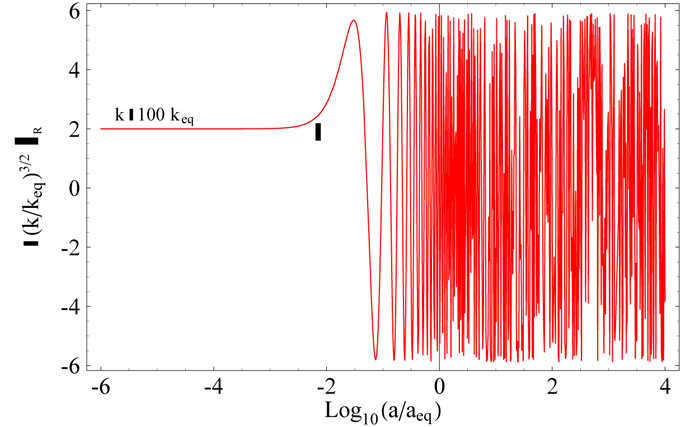Figure 3. Evolution of R for a mode with k = 100 keq. The mode remains frozen outside the Hubble radius at (k / keq)3/2(-R) (k / keq)3/2 2 = 2 (in the normalisation used in Fig. 2 ) and oscillates when it enters the Hubble radius. The oscillations are well described by Eq. (80) with an amplitude of 6.

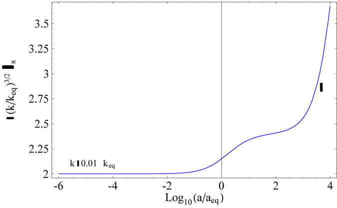Figure 4. Evolution of R for two modes k = keq and k = 0.01 keq. The modes remain frozen outside the Hubble radius at (-R) 2 and oscillates when it enters the Hubble radius. The mode in the right panel stays outside the Hubble radius for most part of its evolution and hence changes very little.

Figure 5. Evolution of |m| for 3 different modes. The modes are labelled by their wave numbers and the epochs at which they enter the Hubble radius are shown by small arrows. All the modes remain frozen when they are outside the Hubble radius and grow linearly in the matter dominated phase once they are inside the Hubble radius. The mode that enters the Hubble radius in the radiation dominated phase grows logarithmically until y = yeq. These features are well approximated by Eqs. (83), (85).

Let us next consider matter perturbations during this phase. They grow, driven by the gravitational potential determined above. When y << 1, Eq. (73) becomes:

(81)

The is essentially determined by radiation and satisfies Eq. (61); using this, we can rewrite Eq. (81) as

(82)

The general solution to the homogeneous part of Eq. (82) (obtained by ignoring the right hand side) is (c₁ + c₂ lny); hence the general solution to this equation is

(83)

For y << 1 the growing mode varies as lny and dominates over the rest; hence we conclude that, matter, driven by , grows logarithmically during the radiation dominated phase for modes which are inside the Hubble radius.

4.3. Evolution in the matter dominated phase

Finally let us consider the matter dominated phase, in which we can ignore the radiation and concentrate on Eq. (72) and Eq. (73). When y >> 1 these equations become:

(84)

These have a simple solution which we found earlier (see Eq. (69)):

(85)

In this limit, the matter perturbations grow linearly with expansion: _m y a. In fact this is the most dominant growth mode in the linear perturbation theory.

4.4. An alternative description of matter-radiation system

Before proceeding further, we will describe an alternative procedure for discussing the perturbations in dark matter and radiation, which has some advantages. In the formalism we used above, we used perturbations in the energy density of radiation (_R) and matter (_m) as the dependent variables. Instead, we now use perturbations in the total energy density, and the perturbations in the entropy per particle, as the new dependent variables. In terms of _R, _m, these variables are defined as:

	(86)
	(87)

Given the equations for _R, _m, one can obtain the corresponding equations for the new variables (, ) by straight forward algebra. It is convenient to express them as two coupled equations for and . After some direct but a bit tedious algebra, we get:

	(88)
	(89)

where we have defined

(90)

These equations show that the entropy perturbations and gravitational potential (which is directly related to total energy density perturbations) act as sources for each other. The coupling between the two arises through the right hand sides of Eq. (88) and Eq. (89). We also see that if we set = 0 as an initial condition, this is preserved to (k⁴) and - for long wave length modes - the evolves independent of . The solutions to the coupled equations obtained by numerical integration is shown in Fig. (2) right panel. The entropy perturbation 0 till the mode enters Hubble radius and grows afterwards tracking either _R or _m whichever is the dominant energy density perturbation. To illustrate the behaviour of , let us consider the adiabatic perturbations at large scales with 0, k 0; then the gravitational potential satisfies the equation:

(91)

which has the two independent solutions:

(92)

both of which diverge as y 0. We need to combine these two solutions to find the general solution, keeping in mind that the general solution should be nonsingular and become a constant (say, unity) as y 0. This fixes the linear combination uniquely:

(93)

Multiplying by _i we get the solution that was found earlier (see Eq. (78)). Given the form of and 0 we can determine all other quantities. In particular, we get:

(94)

The corresponding velocity field, which we quote for future reference, is given by:

(95)

We conclude this section by mentioning another useful result related to Eq. (88). When 0, the equation for can be re-expressed as

(96)

where we have defined:

(97)

(The i factor arises because of converting a gradient to the k space; of course, when everything is done correctly, all physical quantities will be real.) Other equivalent alternative forms for , which are useful are:

(98)

For modes which are bigger than the Hubble radius, Eq. (96) shows that is conserved. When = constant, we can integrate Eq. (98) easily to obtain:

(99)

This is the easiest way to obtain the solution in Eq. (78).

The conservation law for also allows us to understand in a simple manner our previous result that only deceases by a factor (9/10) when the mode remains bigger than Hubble radius as we evolve the equations from y << 1 to y >> 1. Let us compare the values of early in the radiation dominated phase and late in the matter dominated phase. From the first equation in Eq. (98), [using ' 0 we find that, in the radiation dominated phase, (1/2) _i + _i = (3/2) _i; late in the matter dominated phase, (2/3)_f + _f = (5/3) _f. Hence the conservation of gives _f = (3/5)(3/2)_i = (9/10) _i which was the result obtained earlier. The expression in Eq. (99) also works at late times in the dominated or curvature dominated universe.

One key feature which should be noted in the study of linear perturbation theory is the different amount of growths for , _R and _m. The either changes very little or decays; the _R grows in amplitude only by a factor of few. The physical reason, of course, is that the amplitude is frozen at super-Hubble scales and the pressure prevents the growth at sub-Hubble scales. In contrast, _m, which is pressureless, grows logarithmically in the radiation dominated era and linearly during the matter dominated era. Since the later phase lasts for a factor of 10⁴ in expansion, we get a fair amount of growth in _m.