


Given the importance of cosmic acceleration, is there some way to detect it in itself, rather than through the curves of the expansion history? Recall Figure 3. There we motivated the Equivalence Principle by showing how acceleration equals gravity. We can detect the acceleration through the cosmological version of the gravitational redshift. Photons (or any signal) will have their frequencies shifted by the acceleration just as they would by a gravitational field. Of course the expansion of space in itself redshifts photons, but that is analogous to a velocity or Doppler shift; acceleration will add a second time derivative of the photon frequency, showing up a drift in the redshift z.
The redshift drift was first discussed by [6] and given in general form by [7]. Analysis of its use as a cosmological probe, including observational challenges and systematics, appeared in [8, 9]. The result is that
 |
(3) |
where H =  / a is the Hubble parameter and H0 is the present
expansion rate, the Hubble constant. Since the scale factor
a = 1 / (1 + z)
we clearly see that
/ a is the Hubble parameter and H0 is the present
expansion rate, the Hubble constant. Since the scale factor
a = 1 / (1 + z)
we clearly see that  vanishes only in universes with
= constant. That is,
redshift drift is a direct
signature of acceleration (or deceleration). However, since the Hubble
time H-1 is more than 10 billion years,
the redshift drifts at only 1 part in 1010 per year, beyond
present
technology to measure. Even with a 20 year observational program with
stability achieved at the one part in a billion level, the cosmological
leverage of such a measurement is unimpressive. Moreover, as
[8,
9,
10]
pointed out, just as peculiar velocities interfere with accurate redshift
measurements, so would peculiar accelerations degrade redshift drift.
These can take the form of endpoint effects, i.e. jitter in the observer
or source motion due to realistically inhomogeneous gravitational fields
from mass flows, or propagation effects such as a stochastic
gravitational wave background with energy density as small as
10-17 of critical density would generate significant noise.
vanishes only in universes with
= constant. That is,
redshift drift is a direct
signature of acceleration (or deceleration). However, since the Hubble
time H-1 is more than 10 billion years,
the redshift drifts at only 1 part in 1010 per year, beyond
present
technology to measure. Even with a 20 year observational program with
stability achieved at the one part in a billion level, the cosmological
leverage of such a measurement is unimpressive. Moreover, as
[8,
9,
10]
pointed out, just as peculiar velocities interfere with accurate redshift
measurements, so would peculiar accelerations degrade redshift drift.
These can take the form of endpoint effects, i.e. jitter in the observer
or source motion due to realistically inhomogeneous gravitational fields
from mass flows, or propagation effects such as a stochastic
gravitational wave background with energy density as small as
10-17 of critical density would generate significant noise.
As for dynamical effects of dark energy within the solar system or
astrophysical systems, the energy density is simply too low. All the
dark energy within the entire solar system constitutes the energy
equivalent of three hours of sunlight at 1 AU, ruling out any direct
effect on orbits. For lensing by black holes, say, the relative
contribution to the deflection of light by a cosmological constant
 is
r2 / (m / r).
Detectable lensing requires a gravitational potential
is
r2 / (m / r).
Detectable lensing requires a gravitational potential
 ~ m / r
 10-6, and
~
H2 so it would require a black hole with
mass greater than 1013
M
10-6, and
~
H2 so it would require a black hole with
mass greater than 1013
M before
dark energy would contribute
even 1% effect - and at that point the static approximation used here
breaks down. Thus, cosmological expansion remains the practical path to
mapping acceleration.
before
dark energy would contribute
even 1% effect - and at that point the static approximation used here
breaks down. Thus, cosmological expansion remains the practical path to
mapping acceleration.
It is attractive to consider how much information one can extract on the expansion history from minimal assumptions. If one uses only the geometry of spacetime as an input, i.e. the Robertson-Walker metric, then one can learn a remarkable amount. For example, the expansion of space and redshift of photons, hence the decrease in temperature and density as the universe expands, are directly derived from examination of the metric. Such properties that do not rely on supplementing the geometry with equations of motion are referred to as kinematics, while those that depend on the field equations, i.e. the specific theory of gravity, fall under dynamics.
For example, the relation between conformal distance
 and the
expansion factor a is kinematic,
and the
expansion factor a is kinematic,
 |
(4) |
but if H is defined in terms of
, i.e.
H =
/ a = a-2da /
d,
then this becomes a tautology. To actually evaluate the distance-redshift
relation requires a model for H, generally supplied by the
equations of motion, that is the Friedmann equations in terms of the
densities and pressures. Before returning to this, let us consider
kinematic signatures of acceleration.
In the diagrams of Figure 1,
acceleration would show up
as convexity of the curves, i.e. the second derivative becomes positive.
A clearer and more direct way of seeing acceleration is by transforming
the variables plotted to the conformal horizon scale as a function of
expansion factor; see Figure 4. A size of the
visible universe can be defined in terms
of the Hubble length, H-1, where the expansion, or
e-folding, rate H =
/ a. Since all lengths expand with the scale factor a, we
can transform into conformal, or comoving, coordinates by dividing by
a, thus defining the conformal horizon scale
(aH)-1.
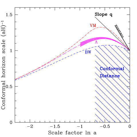 |
Figure 4. This conformal history diagram
presents a unified picture of
important properties of the cosmic expansion. Curves represent the
expansion history of different cosmological models (here the cosmological
constant |
Comoving wavelengths would appear as horizontal lines in this plot and
so wavelengths enter the horizon, i.e. fall below the horizon history
curve, at early times as the universe expands. For decelerating expansion,
this is the whole story, with more wavemodes being revealed as the
expansion continues. However, for accelerating universes, the slope of
the horizon history curve goes negative and modes can leave the horizon.
This condition d(aH)-1 / d lna ~
-  < 0 and its
consequences are precisely the principle behind inflation: an
accelerating epoch in the early universe.
< 0 and its
consequences are precisely the principle behind inflation: an
accelerating epoch in the early universe.
This diagram demonstrates visually the tight connection between the expansion history (the value along the curve), acceleration (the slope of the curve), and distances of objects in the universe (the area under the curve). Thus distances provide a clear and direct method for mapping the expansion history, and will be treated at length in Section 3.
However, as stated above, to actually evaluate the curve for an expansion
history one needs a model for the expansion. One could adopt an ad hoc
model a(t) or H(z) or, parameterizing the
acceleration directly, q(z) where q = -a
/
2 is called
the deceleration parameter, or
even the third derivative j = a2
/
3 called the
jerk. One runs the danger of substituting the physics of the Einstein
equations with some other, implicit dynamics since adopting a form for
q(z) is equivalent to some ad hoc equation of
motion. Explicitly, if one defines H2 =
f( ),
some function of the total density, say, then the continuity equation leads
to q = -1 + (3/2)(1 + w) d ln f / d
ln , so
choosing some functional form
q(z), or j(z), is choosing an
equation of motion. That is, one has not truly achieved kinematic
constraints, only substituted some other unspecified physics for general
relativity.
),
some function of the total density, say, then the continuity equation leads
to q = -1 + (3/2)(1 + w) d ln f / d
ln , so
choosing some functional form
q(z), or j(z), is choosing an
equation of motion. That is, one has not truly achieved kinematic
constraints, only substituted some other unspecified physics for general
relativity.
One method for getting around this is by putting no physics into the form by taking a Taylor expansion, e.g. q(z) = q0 + q1z [11, 12]. This has limited validity, that is it can only be applied to mapping the expansion at very low redshifts z << 1 and it is not clear what has actually been gained. Another method is to allow the data to determine the form, and the physics, through principal component analysis as in [13, 12]. This has a broader range of physical validity, but has substantial sensitivity to noise in the data, since it seeks to extract information on a third derivative in the case of jerk.
Einstein's equations provide the dynamics in terms of the energy-momentum
components in the universe. Note that alterations to the form of the
gravitational
action also define the dynamics. Unless otherwise specified we consider
Friedmann-Robertson-Walker cosmologies. In this case, the simplest
ingredients are the energy density and pressure of each component, with
the components assumed to be noninteracting. This can be phrased
alternately in terms of the present dimensionless energy density
 w
= 8
w
= 8 Gw(z = 0) /
(3H02) and the pressure to density, or
equation of state, ratio w = pw /
w.
Gw(z = 0) /
(3H02) and the pressure to density, or
equation of state, ratio w = pw /
w.
We have seen in Section 1.2 that the equation of state is central to the relation between geometry and destiny, and it plays a key role in the dynamics of the expansion history as well. In Figure 5 we see the very different behaviors for the dark energy density for different classes of equations of state. The cosmological constant has an unchanging energy density, and so it defines a unique scale, tiny in comparison to the Planck energy, and a particular time in cosmic history when it is comparable to the matter density. These fine tunings give rise to the cosmological constant problem [14, 15, 16]. Dynamical scalar fields, called quintessence, change their energy density and this may or may not alleviate the large discrepancy with the Planck scale. One of the two main classes of such fields [17], thawing fields that evolve away from early cosmological constant behavior, has energy density that changes little. The other class, freezing fields that evolve toward late time cosmological constant behavior, can have much greater energy density at early times. For example, tracking fields may contribute an appreciable fraction of the energy density over an extended period in the past and may approach the Planck density at early times, while scaling fields mimic the behavior of the dominant energy density component, contributing so much to the dynamics that they can be strongly constrained.
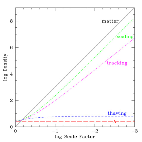 |
Figure 5. In the recent expansion history, matter and dark energy have contributed similar amounts of energy density (shown here normalized to the present matter density) but this is apparently coincidental. Among quintessence models, the energy density of the cosmological constant or a thawing field differs substantially at early times from freezing fields such as trackers or scalers, one example of classification of dark energy models. |
Although there is a diversity of dynamical behaviors [18], these fall into distinct classes of the physics behind acceleration [17]. We see that to reveal the origin of cosmic acceleration we will require precision mapping of the expansion history over the last e-fold of expansion, but we may also need to measure the expansion history at early times. And to predict the future expansion history and the fate of the universe requires truly understanding the nature of the new physics - for example knowing whether dark energy will eventually fade away, restoring the link between geometry and destiny.
Before proceeding further we can ask whether the Robertson-Walker model of a homogeneous, isotropic universe is indeed the proper framework for analyzing the expansion history. Certainly the global dynamics of the expansion follows that of a Friedmann-Robertson-Walker model (FRW), as the successes of Big Bang nucleosynthesis, cosmic microwave background radiation measurements, source counts etc. show [19, 20], but one could imagine smaller scale inhomogeneities affecting the light propagation by which we measure the expansion history. This has long been known [21, 22, 23] and for stochastic inhomogeneities shown to be unimportant in the slow motion, weak field limit [24].
To grasp this intuitively, consider that the expansion rate of space is not a single number but a 3 × 3 matrix over the spatial coordinates. The analog of the Hubble parameter is (one third) the trace of this matrix, so inhomogeneities capable of altering the global expansion so as to mimic acceleration generically lead to changes in the other matrix components. This induces shear or rotation of the same order as the change in expansion, leading to an appreciably anisotropic universe. Observations however limit shear and rotation of the expansion to be less than 5 × 10⁻⁵-10-6 times the Hubble term [25].
Thus, to create the illusion of acceleration one would have to carefully
arrange the material contents of the universe, adjusting the density
along the line of sight (spherical symmetry is not wholly necessary
with current data quality). Again, this has long been discussed
[26,
27,
28]
and indeed changes the distance-redshift relation. The simple model of
[29]
poses the problem in its most basic terms, clearly demonstrating its
meaning. It considers an inhomogeneous, matter only universe with a void
( = 0 for the
Dyer-Roeder smoothness parameter) somewhere along
the line of sight, extending from z1 to
z1 +
= 0 for the
Dyer-Roeder smoothness parameter) somewhere along
the line of sight, extending from z1 to
z1 +
 z,
and finds that the distances to sources lying at higher redshift do not
agree with the FRW relation. Even for very high redshift sources where the
cosmic volume is essentially wholly described by FRW there maintains an
asymptotic fractional distance deviation o
z /
(1 + z1) (if the void surrounds
the observer then the deviation is of order
z2).
z,
and finds that the distances to sources lying at higher redshift do not
agree with the FRW relation. Even for very high redshift sources where the
cosmic volume is essentially wholly described by FRW there maintains an
asymptotic fractional distance deviation o
z /
(1 + z1) (if the void surrounds
the observer then the deviation is of order
z2).
Suppose we were to define w(z) in terms of derivatives of distance with respect to redshift. Then we would find for certain choices of void size and location that w(z) < -1/3; see Figure 6. Apart from the fact that this would require enormous voids, it would be a mistake to interpret this as apparent acceleration within this very basic, matter only model. The analysis is physically inconsistent because it treats the expansion, e.g. H(z), in two different ways: as dynamics, for example in the friction term in the Raychaudhuri or beam equation, and as kinematics, through the correspondence to the differential of the distance, dr / dz ~ H. We emphasize this point: in models with inhomogeneities, it is inconsistent to treat dynamics and kinematics the same. See [30] for further discussion of the proper physical interpretation of acceleration.
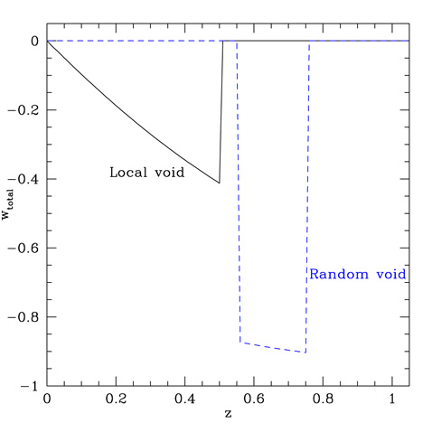 |
Figure 6. Huge voids can give the illusion of an effective negative equation of state and acceleration, but not the dynamical reality. The solid curve gives the effective total equation of state if we observe from the center of a void extending out to z = 0.5, yet interpret data within a smooth FRW model. The dashed curve corresponds to a void in a shell from z = 0.55-0.75. |
While the previous approach can deliver a mirage of, but not physical, acceleration, one cannot even obtain such an illusion if one requires other basic aspects of FRW to hold. From the Raychaudhuri, or beam, equation (see [21]) in FRW generalized to arbitrary components and smoothness [31], one finds the following two conditions,
 |
(5) |
must hold for a pure matter, inhomogeneous model to mimic a smooth model with matter plus an extra component with equation of state w (so the total equation of state is wtot). These follow from matching the Raychaudhuri equation term by term between the models, so that the distance-redshift relations will agree. However, the requirement of positive energy density then immediately demonstrates that an effective wtot < -1/3 cannot be attained, i.e. acceleration is not possible. Moreover, the matter in the inhomogeneous dust model cannot consistently obey the usual continuity equation.
Thus, a pure dust model with inhomogeneities described by spatial under-
and overdensities, i.e.
(z), cannot give
distances matching an
accelerating FRW universe distance-redshift relation, nor any FRW model
without introducing nonstandard couplings in the matter sector.
Finally, to obtain even the mirage of a perfectly isotropic distance-redshift relation requires the inhomogeneities to be arranged in a spherically symmetric manner around the observer, raising issues of our preferred location. If the inhomogeneities are arranged only stochastically, i.e. do not have an infinite coherence length caused by special placement, then the effects along the line of sight will average out and the distance-redshift relation will reflect the true global expansion. Thus, save for hand fashioning a universe to deceive, observed acceleration is real acceleration.
Given accelerated expansion at present, we still cannot absolutely predict the future expansion and the fate of the universe. If the acceleration from dark energy continues then the universe becomes a truly dark, cold, empty place. The light horizon, within which we can receive signals, grows linearly with time, as always, but the particle horizon giving the (at some time) causally influenced region grows more quickly in an accelerating universe (exponentially in the cosmological constant case). Thus, though formally our observational reach out into the universe increases, we see an ever tinier fraction of the causal universe. (See [32] for more on horizons.)
Also, although the light horizon expands, in a real sense the visible universe does "close in" around us not through objects going beyond the horizon but through their fading away to our sight. For example, in a cosmological constant dominated universe the redshift of an object at constant comoving distance increases exponentially with time, so its received flux decreases exponentially and its surface brightness fades exponentially from the usual (1 + z)4 law. Conversely, the comoving distance to a fixed redshift decreases exponentially with time, so vanishingly few objects lie within the volume to any finite redshift and hence have non-infinitesimal flux and surface brightness. (See [33, 34, 5] for some specific calculations.) Thus our view of the universe does not so much shrink as darken. (So dark energy is well named.)
The existence of a horizon arising from acceleration, or Rindler horizon
[35],
brings another set of physics puzzles, best known for the borderline case
of w = -1. In de Sitter space the horizon causes loss of
unitarity and makes it problematic to define particle interaction
probabilities through an S matrix
[14].
On the other hand, the horizon may be instrumental in
obviating the Big Rip fate. For a universe with w < -1 the
increasing (conformal) acceleration overcomes all other binding forces,
ripping planets, atoms, etc. apart
[36].
However, Unruh radiation, or thermal particle creation from the horizon,
with temperature T ~ g and hence energy density
~
T4 where g =
/ a is the
conformal acceleration (so the rip condition
is not  > 0 but
( / a)
. > 0), should quickly overwhelm the dark energy
(whose density increases as g, not g4). Thus
the horizon should act to either decelerate the universe or bring the
expansion to some non-superaccelerating state
[37].
> 0 but
( / a)
. > 0), should quickly overwhelm the dark energy
(whose density increases as g, not g4). Thus
the horizon should act to either decelerate the universe or bring the
expansion to some non-superaccelerating state
[37].
Other possibilities for the fate of the universe include collapse
(a  0)
if the dark energy attains negative values of its potential, as in
the linear potential model
[38]
(also see Section 6.3),
collapse and bounce into new expansion as in the cyclic model
[39],
or eternal but decelerating expansion if the dark energy fades away.
0)
if the dark energy attains negative values of its potential, as in
the linear potential model
[38]
(also see Section 6.3),
collapse and bounce into new expansion as in the cyclic model
[39],
or eternal but decelerating expansion if the dark energy fades away.
Thus we have seen throughout this section that to distinguish the origin
of cosmic acceleration
we may need not only to map accurately the recent expansion
history, but distinguish models of dark energy through their early
time behavior and understand their nature well enough to predict their
future evolution.
To truly understand our universe we must map the cosmic expansion from
a = 0 to a =  - and possibly back to a = 0 again.