


This section is somewhat pedagogical in nature, containing a brief summary of the work of Bondi, Hoyle and Lyttleton. Readers familiar with the basic nature of Bondi-Hoyle-Lyttleton accretion may wish to skip this section.
2.1. The Analysis of Hoyle & Lyttleton
Hoyle and Lyttleton (1939) considered accretion by a star moving at a steady speed through an infinite gas cloud. The gravity of the star focuses the flow into a wake which it then accretes. The geometry is sketched in figure 1.
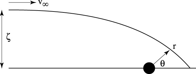 |
Figure 1. Sketch of the Bondi-Hoyle-Lyttleton accretion geometry |
Hoyle and Lyttleton derived the accretion rate in the following manner:
Consider a streamline with impact parameter
 .
If this follows a ballistic orbit (it will if pressure effects are
negligible), then we can apply conventional orbit theory. We have
.
If this follows a ballistic orbit (it will if pressure effects are
negligible), then we can apply conventional orbit theory. We have
 |
(1) (2) |
in the radial and polar directions respectively.
Note that the second equation expresses the conservation
of angular momentum.
Setting h =
v and making the usual
substitution u = r-1, we may rewrite the first
equation as
and making the usual
substitution u = r-1, we may rewrite the first
equation as
 |
(3) |
The general solution is u = A
cos + B
sin + C
for arbitrary constants A, B and C.
Substitution of this general solution immediately shows that
C = GM / h2.
The values of A and B are fixed by the boundary conditions
that u
+ B
sin + C
for arbitrary constants A, B and C.
Substitution of this general solution immediately shows that
C = GM / h2.
The values of A and B are fixed by the boundary conditions
that u  0
(that is, r
) as
0
(that is, r
) as
 , and that
 |
These will be satisfied by
 |
(4) |
Now consider when the flow encounters the
= 0 axis.
As a first approximation, the
velocity will go to zero
at this point. The radial velocity will be
v and the radius of
the streamline will be given by
 |
(5) |
Assuming that material will be accreted if it is bound to the star we have
 |
or
 |
(6) |
which defines the critical impact parameter, known as the Hoyle-Lyttleton radius. Material with an impact parameter smaller than this value will be accreted. The mass flux is therefore
 |
(7) |
which is known as the Hoyle-Lyttleton accretion rate.
The Hoyle-Lyttleton analysis contains no fluid effects, which makes it ripe for analytic solution. This was performed by Bisnovatyi-Kogan et al. (1979), who derived the following solution for the flow field:
 |
(8) (9) (10) (11) |
The first three equations are fairly straightforward, and follow (albeit tediously) from the orbit solution given above. The equation for the density is rather less pleasant, and involves solving the steady state gas continuity equation under conditions of axial symmetry.
Equation 4 may be rewritten into the form
 |
(12) |
where e is the eccentricity of the orbit, r0 is
the semi-latus rectum, and
0 is the
periastron angle. These quantities may be expressed as
 |
(13) (14) (15) |
which may be useful as an alternative form to equation 10.
Note that these equations do not follow material down to the accretor.
Accretion is assumed to occur through an infinitely thin, infinite density
column on the = 0 axis.
This is not physically consistent with the ballistic assumption, since
it would not be possible to radiate away the thermal energy released
as the material loses its
velocity.
Even with a finite size for the accretion column, a significant trapping
of thermal energy would still be expected.
For now we shall neglect this effect.
2.3. The Analysis of Bondi and Hoyle
Bondi and
Hoyle (1944)
extended the analysis to include
the accretion column (the wake following the point mass on the
= 0 axis).
We will now follow their reasoning, and show that this suggests
that the accretion rate could be as little as half the value
suggested in equation 7.
Figure 2 sketches the quantities we shall use.
 |
Figure 2. Sketch of the geometry for the Bondi-Hoyle analysis |
From the orbit equations, we know that material encounters
the = 0 axis at
 |
This means that the mass flux arriving in the distance r to r + dr is given by
 |
(16) |
which defines  .
Note that it is independent of r.
The transverse momentum flux in the same interval is given by
.
Note that it is independent of r.
The transverse momentum flux in the same interval is given by
 |
which is the mass flux, multiplied by the transverse velocity, divided over the approximate area of the wake. Applying the orbit equations once more, and noting that a momentum flux is the same as a pressure, we find
 |
(17) |
as an estimate of the pressure in the wake. The longitudinal pressure force is therefore
 |
Material will take a time of about r /
v to fall onto the
accretor from the point it encounters the axis.
This means that we can use the accretion rate to estimate the mass
per unit length of the wake, m, as
 |
(18) |
This makes the gravitational force per unit length
 |
For accreting material, we must have r ~ G M
v-2.
If we also assume that the wake is thin (s
<< r) and roughly conical (ds / s
 dr /
r), then
taking the ratio of the pressure and gravitational forces, we find
that pressure force is much less than the gravitational force.
We can therefore neglect the gas pressure in the wake.
dr /
r), then
taking the ratio of the pressure and gravitational forces, we find
that pressure force is much less than the gravitational force.
We can therefore neglect the gas pressure in the wake.
The mass per unit length of the wake, m, was introduced above. If we assume the mean velocity in the wake is v, we can write two conservation laws, for mass and momentum:
 |
(19) (20) |
Recall that
v is the momentum supply
into the wake, since r =
v on axis for all streamlines.
We can declutter these equations by introducing dimensionless
variables for m, r and v:
 |
(21) (22) (23) |
Note that  =
2 corresponds to material arriving from the streamline
characterised by
HL.
Substituting these definitions into equations 19 and 20, we obtain
=
2 corresponds to material arriving from the streamline
characterised by
HL.
Substituting these definitions into equations 19 and 20, we obtain
 |
(24) (25) |
We shall now analyse the behaviour of these equations.
We can integrate equation 24 to yield
 |
(26) |
for some constant  .
Since µ is a scaled mass (and hence always positive), we see
that the scaled velocity
(
.
Since µ is a scaled mass (and hence always positive), we see
that the scaled velocity
( ) changes sign when
=
.
That is, is the
stagnation point.
Material for
<
will accrete, so knowing
will
tell us the accretion rate (since the accretion rate will be
r0
where r0 is the value of r
corresponding to ).
By writing
µ2 =
µ ·
, we can use
equation 26 to rewrite equation 25 as
) changes sign when
=
.
That is, is the
stagnation point.
Material for
<
will accrete, so knowing
will
tell us the accretion rate (since the accretion rate will be
r0
where r0 is the value of r
corresponding to ).
By writing
µ2 =
µ ·
, we can use
equation 26 to rewrite equation 25 as
 |
(27) |
This has not obviously improved matters, but we can now study the general behaviour of the function, without trying to solve it. First we need some boundary conditions. These are as follows:
1 as
v at large radii
= 0 at
=
/
d > 0 Everywhere
The velocity must be a monotonic function. This is physically reasonable, if we are to avoid unusual flow patterns
The first two conditions can be satisfied for any value of
.
Fortunately, the third implies as restriction.
The next set of manipulations may seem a little obscure at first, but
they do lead in the desired direction.
Substitute  =
-1
.
Equation 27 then reads
=
-1
.
Equation 27 then reads
 |
(28) |
Now, suppose the derivative is zero. This leads to the condition
 |
or, one application of the quadratic roots formula later:
 |
(29) |
Since ultimately represents a
physical quantity (the velocity), it's obviously desirable that it
remain real. We therefore need to look at when the discriminant can
become zero. This is another quadratic equation, leading to
 |
which means that something must happen when
= 1.
To determine this `something,' it is best to plot equation 29.
Figures 3 and 4
demarcate the regions where d
/ d changes
sign, as dictated by equation 29. These are not possible
solutions for .
However, any suitable solution for
must remain within
the region marked `a' if it is to remain monotonic and increasing.
This is only possible when
> 1.
Unwinding our rescaled variables, we see that an
value
of unity puts the stagnation point halfway between the accretor
and the original value of Hoyle and Lyttleton.
This in turn implies a minimum accretion rate of 0.5 MHL.
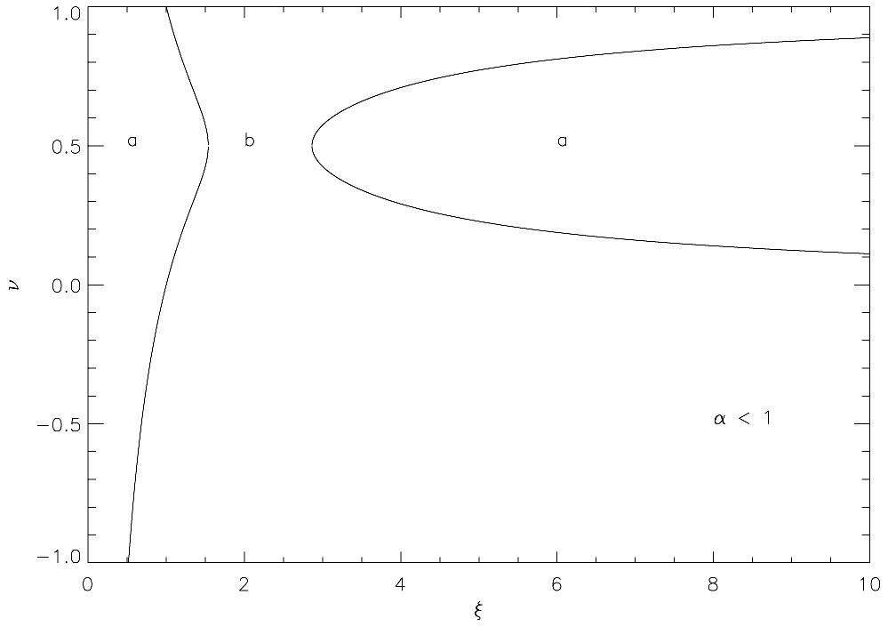 |
Figure 3. Curves where
d |
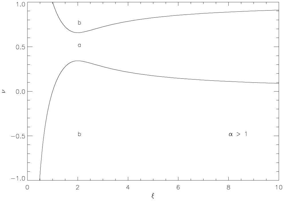 |
Figure 4. Curves where
d |
Again, I would like to remind the reader that the flow has been
assumed to remain isothermal with negligible gas pressure
throughout this discussion. This assumption is likely to be violated in
the wake, where densities will be high and radiative heat loss inefficient.
At the very least, thermal effects should be important close
to the stagnation point in the wake.
Horedt
(2000)
details an analysis similar to that
given above, but with a pressure term included.
The value of (which
Horedt calls
x0) was found to lie between 0.6 and 3.5 for flows which
were supersonic at infinity and subject to Newtonian physics
(the polytropic and adiabatic indices were also free parameters
in this analysis).
Will the flow be stable?
Bondi and Hoyle asserted that
if > 2 (note that
= 2 gives the solution of
Hoyle and Lyttleton), then the wake would become unstable to
perturbations which preserve axial symmetry. However, later analysis by
Cowie
(1977)
suggested that the wake should be unstable, regardless of the value
of .
Subsequent numerical simulations and analytic work have shown
that Bondi-Hoyle-Lyttleton flow is far from stable, and
we will discuss the subject in section 4.2.
2.4. Connection to Bondi Accretion
Bondi (1952) studied spherically symmetric accretion onto a point mass. The analysis shows (see e.g. Frank et al. (2002)) that a Bondi radius may be defined as
 |
(30) |
Flow outside this radius is subsonic, and the density is almost uniform. Within it, the gas becomes supersonic and moves towards a freefall solution. The similarities between equations 6 and 30 led Bondi to propose an interpolation formula:
 |
(31) |
This is often known as the Bondi-Hoyle accretion rate. On the basis of their numerical calculations, Shima et al. (1985) suggest that equation 31 should acquire an extra factor of two, to become
 |
(32) |
which then matches the original Hoyle-Lyttleton rate as the sound
speed becomes insignificant. The corresponding
BH
is formed by analogy with equation 7.
Nomenclature in this field can be a little confused.
When papers refer to `Bondi-Hoyle accretion rates,' they may mean
equation 7, 31 or 32. In this review, I shall refer to pressure-free
flow as `Hoyle-Lyttleton' accretion and use MHL and
HL.
When there is gas pressure, I will talk about `Bondi-Hoyle accretion' and
use MBH and
BH,
in the sense defined by equation 32. I shall use `Bondi-Hoyle-Lyttleton'
accretion to refer to the problem in general terms.