2. LMC KINEMATICS

Kinematical observations for the LMC have been obtained for many tracers. The kinematics of gas in the LMC has been studied primarily using HI (e.g., Kim et al. 1998; Olsen & Massey 2007). Discrete LMC tracers which have been studied kinematically include star clusters (e.g., Schommer et al. 1992; Grocholski et al. 2006), planetary nebulae (Meatheringham et al. 1988), HII regions (Feitzinger, Schmidt-Kaler & Isserstedt 1977), red supergiants (Olsen & Massey 2007), red giant branch (RGB) stars (Zhao et al. 2003; Cole et al. 2005), carbon stars (e.g., van der Marel et al. 2002; Olsen & Massey 2007) and RR Lyrae stars (Minniti et al. 2003; Borissova et al. 2006). For the majority of tracers, the line-of-sight velocity dispersion is at least a factor ~ 2 smaller than their rotation velocity. This implies that on the whole the LMC is a (kinematically cold) disk system.

2.1. General Expressions

To understand the kinematics of an LMC tracer population it is necessary to have a general model for the line-of-sight velocity field that can be fit to the data. All studies thus far have been based on the assumption that the mean streaming (i.e., the rotation) in the disk plane can be approximated to be circular. However, even with this simplifying assumption it is not straightforward to model the kinematics of the LMC. Its main body spans more than 20° on the sky and one therefore cannot make the usual approximation that "the sky is flat" over the area of the galaxy. Spherical trigonometry must be used, which yields the general expression (van der Marel et al. 2002; hereafter vdM02):

(1)

with

(2)

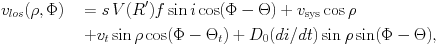
v_los is the observed component of the velocity along the line of sight. The quantities (, ) identify the position on the sky with respect to the center: is the angular distance and is the position angle (measured from North over East). The kinematical center is at the center of mass (CM) of the galaxy. The quantities (v_sys, v_t, _t) describe the velocity of the CM in an inertial frame in which the sun is at rest: v_sys is the systemic velocity along the line of sight, v_t is the transverse velocity, and _t is the position angle of the transverse velocity on the sky. The angles (i, ) describe the direction from which the plane of the galaxy is viewed: i is the inclination angle (i = 0 for a face-on disk), and is the position angle of the line of nodes (the intersection of the galaxy plane and the sky plane). The velocity V(R') is the rotation velocity at cylindrical radius R' in the disk plane. D₀ is the distance to the CM, and f is a geometrical factor. The quantity s = ± 1 is the `spin sign' that determines in which of the two possible directions the disk rotates.

The first term in equation (1) corresponds to the internal rotation of the LMC. The second term is the part of the line-of-sight velocity of the CM that is seen along the line of sight, and the third term is the part of the transverse velocity of the CM that is seen along the line of sight. For a galaxy that spans a small area on the sky (very small ), the second term is simply v_sys and the third term is zero. However, the LMC does not have a small angular extent and the inclusion of the third term is particularly important. It corresponds to a solid-body rotation component that at most radii exceeds in amplitude the contribution from the intrinsic rotation of the LMC disk. The fourth term in equation (1) describes the line-of-sight component due to changes in the inclination of the disk with time, as are expected due to precession and nutation of the LMC disk plane as it orbits the Milky Way (Weinberg 2000). This term also corresponds to a solid-body rotation component.

The general expression in equation (1) appears complicated, but it is possible to gain intuitive insight by considering some special cases. Along the line of nodes one has that sin ( - ) = 0 and cos( - ) = ± 1, so that

(3)

Here it has been defined that _los v_los - v_sys cos v_los - v_sys. The quantity v_tc v_t cos(_t - ) is the component of the transverse velocity vector in the plane of the sky that lies along the line of nodes; similarly, v_ts v_t sin(_t - ) is the component perpendicular to the line of nodes. Perpendicular to the line of nodes one has that cos( - ) = 0 and sin ( - ) = ± 1, and therefore

(4)

Here it has been defined that w_ts = v_ts + D₀ (di / dt). This implies that perpendicular to the line of nodes _los is linearly proportional to sin. By contrast, along the line of nodes this is true only if V(R') is a linear function of R'. This is not expected to be the case, because galaxies do not generally have solid-body rotation curves; disk galaxies tend to have flat rotation curves, at least outside the very center. This implies that, at least in principle, both the position angle of the line of nodes and the quantity w_ts are uniquely determined by the observed velocity field: is the angle along which the observed _los are best fit by a linear proportionality with sin, and w_ts is the proportionality constant.

2.2. Carbon Star Kinematics

vdM02 were the first to fit the velocity field expression in equation (1) in its most general form to a large sample of discrete LMC velocities. They modeled the data for 1041 carbon stars, obtained from the work of Kunkel, Irwin & Demers (1997) and Hardy, Schommer & Suntzeff (unpublished). The combined dataset samples both the inner and the outer parts of the LMC, although with a discontinuous distribution in radius and position angle. Figure 1 shows the data, with the best model fit overplotted. Overall, the model provides a good fit to the data. Olsen & Massey (2007) recently remodeled the same carbon star data (for which they obtained a similar fit as vdM02), as well as a large sample of red supergiant stars.

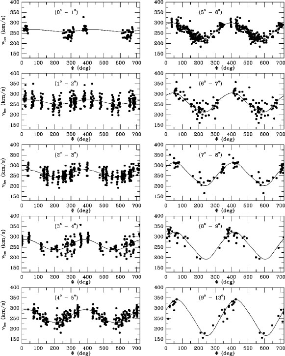Figure 1. Carbon star line-of-sight velocity data from Kunkel et al. (1997) and Hardy et al. (unpublished), as a function of position angle on the sky. The displayed range of the angle is 0°-720°, so each star is plotted twice. Each panel corresponds to a different range of angular distances from the LMC center, as indicated. The curves show the predictions of the best-fitting circularly-rotating disk model from vdM02.

2.3. Viewing Angles and Ellipticity

The LMC inclination cannot be determined kinematically, but the line-of-nodes position angle can. vdM02 obtained = 129.9° ± 6.0° for carbon stars, whereas Olsen & Massey (2007) obtained = 145.3° for red supergiants.

A more robust way to determine the LMC viewing angles is to use geometrical considerations, rather than kinematical ones (since this avoids the assumption that the orbits are circular). For an inclined disk, one side will be closer to us than the other. Tracers on that one side will appear brighter than similar tracers on the other side. To lowest order, the difference in magnitude between a tracer at the galaxy center and a similar tracer at a position (, ) in the disk (as defined in Section 2.1) is

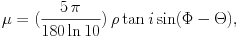(5)

where the angular distance is expressed in degrees. The constant in the equation is (5) / (180ln10) = 0.038 magnitudes. Hence, when following a circle on the sky around the galaxy center one expects a sinusoidal variation in the magnitudes of tracers. The amplitude and phase of the variation yield estimates of the viewing angles (i, ).

Van der Marel & Cioni (2001) used a polar grid on the sky to divide the LMC area into several rings, each consisting of a number of azimuthal segments. The data from the DENIS and 2MASS surveys were used for each segment to construct near-IR color-magnitude diagrams (CMDs). For each segment both the modal magnitude of carbon stars (selected by color) and the magnitude of the RGB tip (TRGB) were determined. This revealed the expected sinusoidal variations at high significance, implying viewing angles i = 34.7° ± 6.2° and = 122.5° ± 8.3°. There is an observed drift in the center of the LMC isophotes at large radii which is consistent with this result, when interpreted as a result of viewing perspective (van der Marel 2001). Also, Grocholski et al. (2006) found that the red clump distances to LMC star clusters are consistent with a disk-like configuration with these same viewing angles.

The aforementioned analyses are sensitive primarily to the structure of the outer parts of the LMC. Several other studies of the viewing angles have focused mostly on the region of the bar, which samples only the central few degrees. Nikolaev et al. (2004) analyzed a sample of more than 2000 Cepheids with lightcurves from MACHO data and obtained i = 30.7° ± 1.1° and = 151.0° ± 2.4°. Persson et al. (2004) obtained i = 27° ± 6° and = 127° ± 10° from a much smaller sample of 92 Cepheids. Olsen & Salyk (2002) obtained i = 35.8° ± 2.4° and = 145° ± 4° from an analysis of variations in the magnitude of the red clump.

In summary, all studies agree that i is approximately in the range 30°-35°, whereas appears to be in the range 120°-150°. The variations between results from different studies may be due to a combination of systematic errors, spatial variations in the viewing angles (warps and twists of the disk plane; van der Marel & Cioni 2001; Olsen & Salyk 2002; Subramaniam 2003; Nikolaev et al. 2004) combined with differences in spatial sampling between studies, contamination by possible out of plane structures, and differences between different tracer populations.

The LMC consists of an outer body that appears elliptical in projection on the sky, with a pronounced, off-center bar. The appearance in the optical wavelength regime is dominated by regions of strong star formation, and patchy dust absorption. However, when only RGB and carbon stars are selected from near-IR surveys such as 2MASS, the appearance of the LMC morphology is actually quite regular and smooth, apart from the central bar. Van der Marel (2001) found that at radii r 4° the contour shapes converge to an approximately constant position angle PA_maj = 189.3° ± 1.4° and ellipticity = 0.199 ± 0.008. A disk that is intrinsically circular will appear elliptical in projection on the sky, with the major axis position angle PA_maj of the projected body equal to the line-of-nodes position angle . The fact that for the LMC PA_maj implies that the LMC cannot be intrinsically circular. When the LMC viewing angles are used to deproject the observed morphology, this yields an in-plane ellipticity in the range ~ 0.2-0.3. This is larger than typical for disk galaxies, and is probably due to tidal interactions with either the SMC or the Milky Way.

2.4. Transverse Motion and Kinematical Distance

As discussed in Section 2.1, the line-of-sight velocity field constrains the value of w_ts = v_ts + D₀ (di / dt). The carbon star analysis in vdM02 yields w_ts = -402.9 ± 13.0 km s^-1. With the assumptions of a known LMC distance D₀ = 50.1 ± 2.5 kpc (based on the distance modulus m - M = 18.50 ± 0.10 adopted by Freedman et al. 2001 on the basis of a review of all published work) and a constant inclination angle with time (di / dt = 0) this yields an estimate of one component of the LMC transverse velocity. Some weaker constraints can also be obtained for the second component. The resulting region in LMC transverse velocity space implied by the carbon star velocity field is shown in Figure 8 of vdM02. This region is entirely consistent with the Hubble Space Telescope (HST) proper motion determination discussed in Section 4.1 below, and therefore provides an important consistency check on the latter. Alternatively, one can use the HST proper motion determination with the measured w_ts and the assumption that di / dt = 0 to obtain a kinematic distance estimate for the LMC. This yields m-M = 18.57 ± 0.11, quite consistent with the Freedman et al. (2001) value.

Previous proper motion estimates for the LMC were lower than the current HST measurements. This introduced artifacts in previous analyses of the internal LMC velocity field (which ultimately depends on subtraction of the v_t term in eq. [1] from the observed line-of-sight velocity field). For example, the HI velocity field of the LMC presented by Kim et al. (1998) showed a pronounced S-shape in the zero-velocity contour. Olsen & Massey recently showed that this S-shape straightens out when the LMC HST proper motion measurement is used instead. So this too provides an independent consistency check on the validity of the HST proper motion measurement.

2.5. Rotation Curve and Mass

The rotation curve of the LMC rises approximately linearly to R' 4 kpc, and stays roughly flat at a value V_rot beyond that. The carbon star analysis of vdM02 with the HST proper motion measurement yields V_rot = 61 km s^-1. By contrast, for HI one obtains V_rot = 80 km s^-1 and for red supergiants V_rot = 107 km s^-1 (Olsen & Massey 2007). The random errors on these numbers are only a few km/s in each case, due to the large numbers of independent velocity samples. Piatek et al. (2008; hereafter P08) recently argued for an even higher V_rot = 120 ± 15 km s^-1 based on rotation measurements in the plane of the sky (based on the same proper motion observations discussed in Section 4.1 below). All of these measurements are influenced by uncertainties in the LMC inclination. However, the uncertainties have different sign for the V_rot values inferred from line-of-sight velocities than and for those inferred from proper motions. The V_rot measurement of P08 becomes more consistent with the line-of-sight measurements if the inclination is lower than the canonical values quoted in Section 2.3. The V_rot estimates from line-of-sight velocities all have an additional uncertainty due to uncertainties in the LMC transverse motion. In the end, all V_rot estimates therefore have a systematic error of ~ 10 km s^-1.

The differences between the V_rot estimates for various tracers are significant, and cannot be attributed to either random or systematic errors. The fact that the HI gas rotates faster than the carbon stars can probably be largely explained as a result of asymmetric drift, with the velocity dispersion of the carbon stars being higher than that of the HI gas (see Section 2.6 below). The difference between the rotation velocities of HI and red supergiants is more puzzling, and may point towards non-equilibrium dynamics. There are in fact clear disturbances in the kinematics of the various tracers (Olsen & Massey 2007). Moreover, the dynamical center of the HI is offset by ~ 1 kpc from the dynamical and photometric center of the stars (see e.g. Cole et al. 2005 for a visual representation of the various relevant centroids of the LMC). All this complicates the inference of the underlying circular velocity of the gravitational potential.

If we use the V_rot of the HI as a proxy for the circular velocity, and use the fact that the carbon star rotation curve remains flat out to the outermost datapoint at ~ 9 kpc, then the implied LMC mass is M_LMC (9 kpc) = (1.3 ± 0.3) × 10¹⁰ M. The mass will continue to rise linearly beyond that radius for as long as the rotation curve remains flat. By contrast, the total stellar mass of the LMC disk is ~ 2.7 × 10⁹ M and the mass of the neutral gas in the LMC is ~ 0.5 × 10⁹ M (Kim et al. 1998). The combined mass of the visible material in the LMC is therefore insufficient to explain the dynamically inferred mass, and the LMC must be embedded in a dark halo.

2.6. Velocity Dispersion and Vertical Structure

As in the Milky Way, younger populations have a smaller velocity dispersion (and hence a smaller scale height) than older populations. Measurements, in order of increasing dispersion, include: ~ 9 km s^-1 for red supergiants (Olsen & Massey 2007); ~ 16 km s^-1 for HI gas (Kim et al. 1998); ~ 20 km s^-1 for carbon stars (vdM02); ~ 25 km s^-1 for RGB stars (Zhao et al. 2003; Cole et al. 2005); ~ 30 km s^-1 for star clusters (Schommer et al. 1992; Grocholski et al. 2006); ~ 33 km s^-1 for old long-period variables (Bessell, Freeman & Wood 1986); ~ 40 km s^-1 for the lowest metallicity red giant branch stars with [Fe/H] < -1.15 (Cole et al. 2005); and ~ 50 km s^-1 for RR Lyrae stars (Minniti et al. 2003; Borissova et al. 2006).

For the stars with the highest dispersions it has been suggested that they may form a halo distribution, and not be part of the LMC disk. On the other hand, this remains unclear, since the kinematics of these stars have typically been observed only in the central region of the LMC. Therefore, it is not known whether the rotation properties of these populations are consistent with being a separate halo component. In fact, the surface density distribution of the LMC RR Lyrae stars is well fit by an exponential with the same scale length as inferred for other tracers known to reside in the disk (Alves 2004). Either way, the vertical extent of all LMC populations is certainly significant. For example, even the (intermediate-age) carbon stars only have V / 3. For comparison, the thin disk of the Milky Way has V / 9.8 and its thick disk has V / 3.9.

The velocity residuals with respect to a rotating disk model do not necessarily follow a Gaussian distribution. Although Zhao et al. (2003) did not find large deviations from a Gaussian for RGB stars, Graff et al. (2000) found that the carbon star residuals are better fit by a sum of Gaussians. More recently, Olsen & Massey (2007) showed that some fraction of both carbon stars and red supergiants have peculiar kinematics that suggest an association with tidally disturbed features previously identified in HI.