


The first procedures to derive the SFH of nearby galaxies from synthetic CMDs were developed by the Bologna and the Padova groups about 20 years ago ([30, 31, 32, 33, 34]), with the latter then combining with the Canary group ([35, 36, 37]). These works used luminosity functions, color distributions and the general CMD morphology to constrain the underlying SFH. In particular, the ratio of star counts in several regions of the CMD was used to determine both the SFR and the IMF ([32]). The drawback of these procedures is the lack of a robust statistical criterion to evaluate the best solution and the corresponding uncertainties. On the other hand, these authors made an optimal use of all the CMD phases and took into careful account all the properties and uncertainties of stellar evolution models, thus avoiding blind statistical approaches, which can lead to misleading results.
Later on, several methods have been proposed to statistically compare simulated and observed CMDs. In this framework, some groups have derived the SFHs of galaxies in the LG, [e.g. [38, 37, 39, 40, 41, 42, 43, 44]]. Others, see e.g. [45, 46, 47, 48], have tackled the question of the SFH in the solar neighborhood. To the same class of investigators we can assign also the study by [49] focused on star clusters. In all these works, the emphasis is transferred from the stellar evolution properties to the problem of selecting the most appropriate model through decision making criteria: here, the likelihood between observed and model CMD is evaluated on statistical bases. There are subtle differences among different groups, reflecting how these authors define the likelihood and how they solve it. The advantages are mainly three: the possibility to exploit each star of the CMD, and not only few strategic ratios; the evaluation of the uncertainty on the retrieved SFH, which is robust; the explorability of a wide parameter space. However, a blind statistical approach is not risk free. Although significant advances have been made in stellar evolution and atmosphere theories, several processes (only to cite the most infamous ones, the HB morphology, RGB and AGB features, convection in general) remain poorly understood and affect the statistical tests. If some parts of the CMDs have a low reliability and others are statistically weak, but very informative (like the helium burning loops), any blind algorithm may miss something crucial. In this case, a careful inspection of the CMD morphology, in particular the ratios of stellar number counts in different evolutionary phases is the irrenounceable and necessary complement to the statistical approach. Finally, whatever the adopted procedure, the absolute rate of star formation must be obtained normalizing the best model to the observed number of stars.
The major differences among the various procedures concern the approach to select the best solutions and the treatment of metallicity variations. In 2001 the predictions of the synthetic CMD method from about ten different groups were compared with each other, showing that, within the uncertainties, most procedures provided consistent results (the Coimbra Experiment: see [50] and references therein).
In the following section we describe the main steps to rank the likelihood among CMDs.
In order to decide if a synthetic CMD is a good representation of the data, the observed and the model star-counts can be compared in a number of CMD regions. In [40] these regions are large and strategically chosen to sample stars of different ages or specific stellar evolutionary phases and to take into account uncertainties in the stellar models: this solution guarantees an optimal statistics, but has the drawback of underexploiting the fine structure of the CMD. Another possibility is to choose a fine grid of regions (see e.g. [51, 52]), counting how many predicted and observed stars fall in each region: the temporal resolution is higher, but the Poisson noise is the new drawback. An intermediate solution is to build a variable grid, coarser where the density of stars is lower and finer when the density is higher (see e.g. [45, 53]). At this level, ad-hoc weighting of some regions can be introduced both to emphasize CMD regions of particular significance for the determination of age, and to mask those regions where stellar evolutionary theory is not robust.
Other authors avoid to grid the CMD: for instance, in [38] each model point (apparent magnitude and color) is replaced with a box with a Gaussian distributed probability density (the photometric error). The total likelihood of a model is the product of the probabilities of observing the data in each box. The idea of this method is equivalent to use blurred isochrones (each point is weighted by the Gaussian spread), so that the photometric uncertainty is embodied in the theoretical model.
The next step is to choose a criterion for the comparison between
synthetic and observational CMDs. For any grid scheme, once binned,
data and synthetic CMDs are converted in color-magnitude
histograms. So, the new problem is to quantify the similarity
among 2D-histograms. One possibility is to minimize a
 2
likelihood function: when the residuals (differences among theoretical
and observed star-counts in the CMD regions) are normally distributed,
all models that have a
2
greater than the best fit plus one are
rejected. However, when the distribution is not normal, a
2
minimization leads to a wrong solution. This motivates the use of the
Poisson likelihood function instead of the least-squares fit-to-data
function. In order to determine the uncertainties around the best
model, a valid alternative is to use a bootstrap test: the original
data are randomly re-sampled with replacements to produce
pseudo-replicated data sets. This mimics the observational process: if
the observational data are representative of the underlying
distribution, the data produced with replacements are copies of the
original one with local crowding or sparseness. The star formation
recovery algorithm is performed on each of these replicated data
sets. The result will be a set of "best" parameters. The confidence
interval is then the interval that contains a defined percentage of
this parameter distribution.
2
likelihood function: when the residuals (differences among theoretical
and observed star-counts in the CMD regions) are normally distributed,
all models that have a
2
greater than the best fit plus one are
rejected. However, when the distribution is not normal, a
2
minimization leads to a wrong solution. This motivates the use of the
Poisson likelihood function instead of the least-squares fit-to-data
function. In order to determine the uncertainties around the best
model, a valid alternative is to use a bootstrap test: the original
data are randomly re-sampled with replacements to produce
pseudo-replicated data sets. This mimics the observational process: if
the observational data are representative of the underlying
distribution, the data produced with replacements are copies of the
original one with local crowding or sparseness. The star formation
recovery algorithm is performed on each of these replicated data
sets. The result will be a set of "best" parameters. The confidence
interval is then the interval that contains a defined percentage of
this parameter distribution.
One aspect deserves closer inspection: the minimization of a merit
function of residuals
(2
or Poisson likelihood) is a global
measure of the fit quality. The first side effect is purely
statistical: low density regions of the CMD may be ignored in the
extremization process, whereas well populated phases (as the MS) are
usually well reproduced. This is a problem of contrast: low density
regions are Poisson dominated, thus, they are much easier to match
with respect to the well populated regions.
A Monte Carlo method can be used with great success to evaluate this bias: building synthetic CMDs from the best set of parameters and re-recovering the SFH can allow to remark any statistical discrepancy. Then, a straightforward solution is to enhance the significance of the discrepant regions of the CMD (with appropriate weights).
Another problem is connected with the theoretical ingredients we have used in the models: first of all, stellar evolution models are not perfect and computations by different groups show systematic differences (see e.g. [54] for a review). Model atmospheres are often unreliable for cool and metal rich stars. Moreover, our models are only covering a part of the possible parameter space and some degree of freedom (additional metallicities, mass loss, overshooting, etc..) may have been neglected. In this case, our best model is only the best (in a relative sense) of the explored parameter space, not necessarily a good one.
In order to deal with these undesirable effects, the residuals can be
placed in the CMD, identifying all the regions where the discrepancy
between observed and predicted star-counts is larger. If the
residuals are larger and concentrated in some part of the CMD, we may
understand what is the reason for the discrepancy and take it into
account. For instance, a poor fit in the red giant branch, less
populated than the main sequence but morphologically well defined in
color (and for this reason often neglected in
2
minimization), may suggest a wrong metallicity, a different mixing
length parameter or wrong color transformations.
3.4. Wondering in the parameter space
The main drawback of Maximum Likelihood (ML) approaches is the computational burden. Algorithms that find the ML score must search through a multidimensional space of parameters, using for instance derivative methods, like Powell's routine, or non-derivative ones, like the downhill simplex routine, or genetic approaches (see e.g. [53]).
These techniques are not guaranteed to find the peak, but work relatively well for a limited number of parameters. Traditionally, this question has been tackled by constructing synthetic CMDs from a SFH built as a series of contiguous bursts and finding the amplitudes of each burst that give the maximum probability to have produced the data: the synthetic CMD is now a linear sum of the partial CMDs produced from a single realization for each burst. In this way a huge parameter space can be explored: rather than calculating a complete CMD for each SFR(t), the partial CMDs can be linearly combined to build a CMD for any SFR(t). In order to reduce the Poisson noise, the partial CMDs are simulated with many more stars than observed (typically, 100 times more).
The computer time spent for building the final CMD is only that needed to go through a finite number of models, simply equal to the number of combinations of Z(t) relations, IMF slopes, reddenings, and distance moduli times the number of age bins in the solution.
Age Bins: Disentangling a stellar population showing both very recent (Myr) and very old (Gyr) episodes of star formation is not straightforward. Only low mass stars survive from ancient episodes because their evolutionary timescales are very long: small CMD displacements, for example due to photometric errors, can bias their age estimates up to some Gyr. In this case, increasing the time resolution, besides being time-consuming, may produce unrealistic star formation rates due to misinterpretations. Hence, the choice of temporal resolution must follow both the time scale of the underlying stellar populations and the data scatter (photometric errors, incompleteness, etc.). A practical way out is to use a coarser temporal resolution for the older epochs, which: 1) allows us to avoid SFH artifacts at early epochs; 2) reduces the Poisson noise; 3) reduces the parameter space. Figure 5 shows a possible time stepping (see [27]). Finally, it's worth noting that the choice of each set of age bins will prevent to identify any SF episode shorter than the bin duration: for instance, the 1 Gyr lull (between 2 and 3 Gyr ago) in the star formation history, as simulated in the top-right panel of Figure 1, will result in a lower (half) activity in the 7th age bin (1-3 Gyr).
 |
Figure 5. Partial theoretical CMDs. Each one is generated with a constant star formation rate, for the age interval pointed out in the label. The bright part of the main sequence is dominated by high mass stars so the CMD time step has to be shorter. |
In the next sections we describe some numerical experiments illustrating the reliability of a typical ML algorithm. In particular, the sensitivity of such algorithm to several physical uncertainties is outlined. These examples expand the discussions and results by [46]. The experiments described here are based on different set of tracks, mass spectrum and photometric errors/completeness, but the results are the same as in [46], thus showing that they are independent of these assumptions. Other instructive examples can be found in [40], [54] and [55].
To describe how a ML procedure works, let's build a fake galaxy assuming for sake of simplicity a constant star formation rate between now and 13 Gyr ago and a metallicity fixed at Z = 0.004. We put it at the distance of the closest dwarf irregular galaxy, the Small Magellanic Cloud (SMC), (m - M)0 = 18.9, and adopt the SMC mean foreground reddening E(B - V) = 0.08. To minimize statistical fluctuations the Monte Carlo extractions are iterated until we have 30000 stars brighter than V = 23, which roughly corresponds to about 100000 stars in the entire CMD. Photometric errors and incompleteness as obtained in actual HST/ACS SMC campaigns [27] are convolved with the synthetic data, producing a realistic artificial population. This fake galaxy will be used as reference set in all the following exercises.
To recover its SFH, we have gridded the CMD in small bins of color and magnitude (0.1 mags large) and we have minimized a Poisson likelihood. The time stepping for the partial CMDs is the following (going backward in time from the present epoch to 13 Gyr ago): 100 Myr, 400 Myr, 500 Myr, 1 Gyr, 2 Gyr, 3 Gyr, 3 Gyr, 3 Gyr. A bootstrap technique is implemented to determine the final uncertainties.
Figure 6 shows on the left-hand panel the CMD of our reference fake galaxy, and on the right-hand panel the SFH recovered from it, using only stars brighter than V = 23 (i.e., MV = 3.85), for a self-consistency check. As expected the retrieved SFR is fitted by a constant value. We will use this basic experiment as starting point for a series of exercises aimed at describing the major uncertainties affecting the synthetic CMD method.
 |
 |
Figure 6. Starting case for the experiments on the uncertainties on the retrieved SFH due to different factors. In the left-hand panel we show an artificial population of stars generated with constant SFR, Salpeter IMF, constant metallicity Z = 0.004 ([23]), (m - M)0 = 18.9, E(B - V) = 0.08 and the HST/ACS errors and completeness of the photometry in the SMC field NGC602 ([27]). In the right-hand panel the input (solid line) and the recovered (dotted) SFH are compared. |
|
3.6. Uncertainties affecting the synthetic CMD procedures
Contrary to real cases, in the reference case of Figure 6 we have all the information: all parameters are known and the data are complete down to 23 (MV = 3.85). Real galaxies are far from this ideal condition. Inadequate information or uncertainty about the assumed parameters can influence the identification of the best SFH. The major sources of uncertainty are primarily the IMF, the binary fraction and the chemical composition. From the observational point of view, the completeness level is another important factor. Moreover, population synthesis methods make a number of simplifications to reduce significantly the computational load; e.g. reddening constant across the data, same distance for all stars, linear age-metallicity relation, etc. Dropping these simplifying assumptions considerably complicates all analyses of the CMD properties.
There are two main strategies to face the complexity of the problem. One is to increase the number of free parameters in the model. For example, [56] recover simultaneously distance, enrichment history and SFR of the local dwarf LGS 3. The other is to reduce the data complexity by means of additional information; for instance, the metallicity may be estimated from appropriate spectroscopy and multi-band observations may help to disentangle the reddening.
In the following sub-sections we test the reliability of the star formation recovery when the uncertainties related to each parameter are taken into account individually. A word of caution is necessary for the interpretation of these exercises: in each case we show how the recovery of the SFH of the reference fake galaxy is affected by forcing the procedure to adopt a specific (and in most cases wrong) value for the tested parameter. This is aimed at emphasizing the effect of that parameter. In the derivations of the SFH of real galaxies, the parameter values are all unknown (which complicates the derivation), but the selection procedure is allowed to cover all the meaningful ranges of values and can therefore distinguish which combinations allow to maximize the agreement with the data.
The numerical experiment seen in section 3.5
represents an
ideal situation: 1) the SMC is one of the closest galaxies, 2) HST/ACS
currently provides the top level photometry in terms of spatial
resolution and depth. At the distance of the SMC (60 kpc), ACS
photometry can be 100% complete to V
 24-25. Farther galaxies
and/or images from ground based telescopes have larger photometric
errors and more severe incompleteness. For comparison, the optical
survey conducted at the Las Campanas Observatory 1 mt Swope Telescope,
to trace the bright stellar population in the Magellanic Clouds, is
50% complete to V ~ 21-22 (see
[57]).
24-25. Farther galaxies
and/or images from ground based telescopes have larger photometric
errors and more severe incompleteness. For comparison, the optical
survey conducted at the Las Campanas Observatory 1 mt Swope Telescope,
to trace the bright stellar population in the Magellanic Clouds, is
50% complete to V ~ 21-22 (see
[57]).
To demonstrate the importance of the completeness limit, we perform the star formation recovery using only stars brighter than V = 21 and V = 22. The results are displayed in Figure 7.
 |
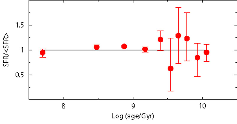 |
Figure 7. Effect of different completeness limits: in the left panel the SFH is recovered using only stars brighter than V=22. In this case, most of the information is still retrieved. In the right panel, this limit is lowered at V=21: as expected, most of the old star formation (older than 1 Gyr) is much more uncertain. |
|
It is evident that the deeper the CMD, the higher the chance to properly derive the old star formation activity. Compared to the V = 23 case, where the SFR recovery is accurate and precise at any age, the quality already drops when the completeness limit is at V = 22: the larger error bars at old epochs reflect the fact that the only signature of the oldest activity comes from evolved stars, less frequent and much more packed in the CMD than the corresponding MS stars. Rising the limiting magnitude at V = 21 further worsens the result, and the recovered SFH is a factor of 2 uncertain for ages older than 1-2 Gyr.
These results are actually optimistic: we have analyzed different levels of completeness with the same photometric errors (HST/ACS), but this is an utopic situation. More distant galaxies have a less favorable completeness limit, and also the photometric error is larger. In these cases, an additional blurring occurs.
A large body of evidence seems to indicate that: 1) the stellar IMF
has a rather universal slope, 2) above 1
M the
IMF is well approximated by a power law with Salpeter-like exponent
[58],
3) below 1
M the
IMF flattens.
the
IMF is well approximated by a power law with Salpeter-like exponent
[58],
3) below 1
M the
IMF flattens.
According to
[28],
the average IMF (as derived from
local Milky Way star-counts and OB associations) is a three-part power
law, with exponent  =
2.7 ± 0.7 for m > 1
M,
= 2.3 ± 0.3 for
0.5 M
< m < 1
M,
= 1.3 ± 0.5 for
0.08 M
< m < 0.5
M. Other
authors, in the past, have proposed different (although somewhat
similar) slopes for the IMF of various stellar mass ranges (e.g.
[59,
60,
29]).
Given these
uncertainties, it is necessary to evaluate how this impacts the
possibility to infer the SFH. In fact, we have the degeneracy condition
that false combinations of IMF and SFH can match as well the
present day mass function (the current distribution of stellar masses)
of MS stars. To quantify it, three fake populations were
generated with different IMF exponents
( = 2, 2.35 and 2.7), but
the SFH searched using always 2.35. The results
are shown in Figure 8.
=
2.7 ± 0.7 for m > 1
M,
= 2.3 ± 0.3 for
0.5 M
< m < 1
M,
= 1.3 ± 0.5 for
0.08 M
< m < 0.5
M. Other
authors, in the past, have proposed different (although somewhat
similar) slopes for the IMF of various stellar mass ranges (e.g.
[59,
60,
29]).
Given these
uncertainties, it is necessary to evaluate how this impacts the
possibility to infer the SFH. In fact, we have the degeneracy condition
that false combinations of IMF and SFH can match as well the
present day mass function (the current distribution of stellar masses)
of MS stars. To quantify it, three fake populations were
generated with different IMF exponents
( = 2, 2.35 and 2.7), but
the SFH searched using always 2.35. The results
are shown in Figure 8.
 |
 |
Figure 8. Effect of different IMFs. SFH recovered assuming Salpeter's IMF exponent (2.35) for synthetic stellar populations actually generated adopting different IMF (labeled in each panel) and a constant SFR. |
|
To interpret these results, one must recall that recent steps of star formation are still populated by the entire mass spectrum, while old steps see only low mass stars because the more massive stars born at those epochs have already died. For old stars a steeper IMF is almost indiscernible from a more intense star formation. In fact, even if evolved stars are included in the SFH derivation, the mass difference between a star at the RGB tip and those at the MS turn-off is only few hundredths of solar masses: too small for allowing the identification of any IMF effect.
For young stars the situation in different. Any attempt to reproduce with an IMF steeper than that of the reference population the number of stars on the lower MS requires a stronger SF activity, but this (wrong) solution leads to overestimating the number of massive stars. Hence, for young stars, IMF and SFH are not degenerate. However, an automatic optimization algorithm, if not allowed to search better solutions including also the IMF among the free parameters, inevitably faces the impossibility to accommodate the number of both massive and low mass stars, by choosing a compromising recent SFH giving higher weight to the more populated (although less reliable) CMD region.
As shown in Fig. 8 the automatic fit tends to overestimate the age of any population whose IMF is actually steeper than the adopted one. And vice versa, for a flatter IMF. Again, we remark that the automatic solution is only the best solution in a parameter space where the IMF is fixed, not necessarily a good one: if the CMD of the recovered SFH is compared with the reference CMD, we immediately recognize that the ratio between low and massive stars is wrong. In other words, to figure out whether our "best" solution is actually acceptable, it is always crucial to compare all its CMD results with the observed one.
Another source of uncertainty is the percentage of stars in unresolved binary systems and the relative mass ratio. The presence of a given percentage of not resolved binary systems affects the CMD morphology. The aim, here, is to see if these effects can destroy or alter the recovered information on the SFH. In order to perform this analysis, we build fake populations using different prescriptions for the binary population (10%, 20% and 30% of binaries with random mass ratio), but the SFH is searched ignoring any binary population (i.e. assuming only single stars). Our models do not include binary evolution with mass exchange, thus we assume that each star in a double system evolves as a single star.
Figure 9 shows the results: as for the IMF, also in this case a modest systematic effect is visible. This is because the stars which are in binary systems are brighter and redder than the average single star population (for an in depth analysis see e.g. [61]). For the recent SFH, this corresponds to moving lower MS stars from a star formation step to the contiguous older step: in this way, the most recent star formation step is emptied of stars, mimicking a lower activity. Intermediate SF epochs are progressively less affected, because some stars get in and some stars get out of the step bin. For the oldest epochs the situation is opposite: the binary effect is to move stars towards younger bins. Here the SGB, that is the main signature of any old population, is brighter because of the binaries, mimicking a younger system.
 |
 |
 |
|
Figure 9. Effect of unresolved binaries. Three fake populations are built with different percentage of binary stars (10%, 20% and 30%). The SFR is recovered using only single stars. |
|
3.10. Metallicity and metallicity spread
The precise position of a star on the CMD depends on the chemical composition, namely the mass fraction of hydrogen, helium and metals (X, Y, Z respectively). The Z content mainly changes the radiative opacity and the CNO burning efficiency: the result of a decreasing Z is to increase the surface temperature and the luminosity of the stars. This has two consequences of relevance for us: a) metal poor stars have a shorter lifetime compared to the metal-rich ones (because over-luminous and hotter), b) a metal-poorer stellar population is bluer, but can be mistaken for a younger but metal-richer population.
To test these effects, the first stars (ages older than 5 Gyr) in our reference fake population are built with a slightly different metallicity (Z = 0.002) than the younger objects, which have the usual Z = 0.004. Then, we recover the SFH by adopting a model with Z = 0.004 independently of age. The results are shown in Figure 10: neglecting that the oldest population of our galaxy was slightly metal poorer, systematic, non negligible discrepancies appear in the recovered SFH. It is the classical age-metallicity degeneracy: to match the blue-shifted sequences of old metal poorer stars, our models with wrong metallicity must be younger. Note that the overall trend of the young SFR is not significantly biased, while the old SFR is now significantly different.
 |
Figure 10. Sensitivity test to metallicity. The reference fake galaxy has a variable composition: Z = 0.004 for stars younger than 5 Gyr, Z = 0.002 for older stars. The red dots represent the SFR as recovered using a single metallicity Z = 0.004 for all epochs. |
This result is a strong warning against any blind attempt to match the CMD with a single (average) metallicity, especially considering that many galaxies exhibit a pronounced age metallicity-relation,
During and at the end of their life stars pollute the surrounding medium, so we expect that more recently formed stars have higher metallicity and helium abundance than those formed at earlier epochs. The progressive chemical enrichment with time results from the combined contribution of stellar yields, gas infall and outflows, mixing among different regions of a galaxy. Observational studies have shown that several galaxies reveal a metallicity spread at each given age.
In
[46]
the SFH sensitivity to a metallicity
dispersion is tested: there several fake populations were generated with
a mean metallicity Z = 0.02 plus a variable dispersion from
 = 0.01 dex to
= 0.2 dex in
[Fe/H]. Then, the SFH was
searched adopting in the model the same mean metallicity of the
artificial data, but without metallicity spread. The results
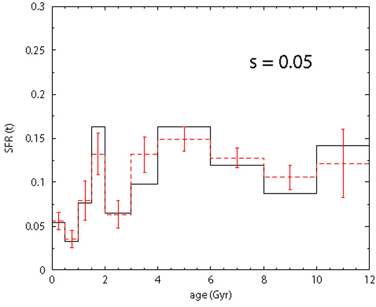
are shown in Fig. 11. Above
= 0.1 dex, the retrieved
SFH differs significantly from the true one: this numerical experiment
points out that the metallicity dispersion can be a non negligible factor.
= 0.01 dex to
= 0.2 dex in
[Fe/H]. Then, the SFH was
searched adopting in the model the same mean metallicity of the
artificial data, but without metallicity spread. The results
are shown in Fig. 11. Above
= 0.1 dex, the retrieved
SFH differs significantly from the true one: this numerical experiment
points out that the metallicity dispersion can be a non negligible factor.
 |
 |
 |
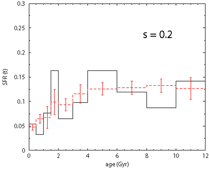 |
Figure 11. Sensitivity test to the
metallicity dispersion. Solid line:
SFH assumed for the fake population. Dashed line: recovered SFH. The
|
|
The SFH retrieval must be also tested against possible variations of the helium abundance for a given metallicity. The abundance of He and metallicity influence the stellar structure through the molecular weight. Increasing Y corresponds to increasing the molecular weight and affects the hydrostatic equilibrium. The pressure decreases and the star shrinks (producing heat), reaching a new equilibrium characterized by a smaller radius and a higher central temperature. As a consequence, the efficiency of the central burning increases and this makes the star brighter and hotter.
Helium absorption lines appear only in the spectra of very hot stars. Hence, the traditional procedure to infer the helium abundance of a standard stellar population cannot be via direct measures and is instead based on the correlation (which is assumed linear) between the helium mass fraction Y and the metal abundance Z.
In order to explore the effects of a wrong choice of the helium content we have built a reference fake population with Z = 0.004 and Y = 0.27 and we have tried to recover its SFH using a Z = 0.004 model coupled with Y = 0.23, which is obviously a very extreme assumption and therefore provides a stringent upper limit to the possible Y effects on the SFH. The result is shown in Figure 12: there are a number of small variations, but the general morphology is well reproduced.
 |
Figure 12. Experiment of the helium effect on the SFH: reference fake population and model have the same metallicity Z = 0.004, but different helium content (Y = 0.23 for the model and Y = 0.27 for the artificial data). The black dashed line is the input SFH. The red solid line is the recovered SFH. |
The small features of the recovered SFR are blended (the peaks are attenuated) but the overall trend is still recovered.
In order to test how wrong choices of reddening and distance
invalidate the possibility to recover the right SFH, we consider two
extreme situations: first, the fake galaxy is put at (m -
M)0 = 18.6, with the models still assuming (m -
M)0 = 18.9; second, the fake
galaxy is reddened using E(B - V) = 0.16 mag, while
the models adopt E(B - V) = 0.08. The results are
shown in Figure 13: it is
evident that the SFH is not recovered, and shows large deviations from
the reference case at any epoch. However, it is worth to remind that
we have derived the best models from a blind
2
minimization: it
is clear that at the distance of SMC, with the beautiful HST
photometry available, both a visual inspection of the CMD morphology
(in particular the blue MS envelope) and the evaluation of the
2
probability would be effective to reject all the models with
wrong distance and reddening. The problem is more challenging for
more distant galaxies, where the only observables are massive stars
and reddening and distance are difficult to constrain.
 |
 |
Figure 13. Sensitivity test to reddening and distance. Red dots represent the recovered SFH. In the left panel the reference fake population is built with a distance spread (m - M)0 = 18.6, while the model used to retrieve the SFH adopts (m - M)0 = 18.9. In the right panel the reference fake population is built with reddening E(B - V) = 0.16, while the model used to retrieve the SFH adopts reddening E(B - V) = 0.08. |
|
Other potential problems are related to differential reddening and line-of-sight depth. There are several indications that some galaxies or portions of them are affected by differential reddening. For instance, young stars can be still surrounded by relics of their birthing cocoon material and suffer an additional amount of absorption. The first signature of a differential reddening is the red clump morphology when it appears elongated and/or tilted (see e.g. [62]). Another effect is a smeared appearance of color and magnitude in any stellar evolution sequence of the CMD.
A finite line-of-sight depth is a natural expectation, at least for nearby galaxies where the physical extension can be a non negligible fraction of their distance from us. As an example, according to [63], the SMC may have a depth of 14-17 kpc, corresponding to a spread in magnitude of few tenths of magnitude. This effect may alter the evolutionary information from the clump and the RGB. A correct description of the stellar populations thus requires analyses involving the spatial structure. Both differential reddening and line-of-sight effects can be dealt with as additional free parameters.
In order to check how the recovered SFH is influenced by differential reddening and line-of-sight spread, we built two fake populations with the following features: the first has a reddening dispersion E(B - V) = 0.08 ± 0.04, the second has a distance spread (m - M)0 = 18.9 ± 0.2. Figure 14 shows the result when the SFH is searched using the canonical combination E(B - V) = 0.08 and (m - M)0 = 18.9. The reference SFH is still fully recovered. The reason is in the random nature of these uncertainties that produce a blurred CMD, but not a systematic trend.
 |
 |
Figure 14. Sensitivity test to differential reddening and line-of-sight spread. Red dots represent the recovered SFH. In the left panel the reference fake population is built with a distance spread (m - M)0 = 18.9 ± 0.2, while the model used to retrieve the SFH has a single distance (m - M)0 = 18.9. In the right panel the reference fake population is built with a differential reddening E(B - V) = 0.08 ± 0.04, while the model used to retrieve the SFH has a single reddening E(B - V) = 0.08. |
|
The previous experiments do not exhaust all the possible sources of uncertainty. Rather, they represent the best understood and manageable ones: among others, convection, atmospheres and color transformations, stellar rotation, mass exchange in binary systems may be relevant as well. Moreover, we have explored each single bias separately, while in a real galaxy several uncertainties may be at work simultaneously with different intensities. In this case, the final effect may not be the simple summation of the previous results: some of the effects may compensate each other or conspire to build an uncertainty larger than the sum of the individual uncertainties.
For example, in the metallicity experiment, when the reference old population was metal poorer than in the search procedure, the retrieved SFH resulted younger. However, this is true only if the best SFH is searched with fixed reddening. Letting the reddening vary could lead to a different SFH (and reddening).
To summarize, the final uncertainty on the recovered SFH strongly depends on which parameter space is explored. Generally speaking, when the best photometric conditions are achieved and all the parameter space is properly covered, within the reached lookback time the error on the epochs of the SF activities is around ten percent of their age and that on the SFR is of the order of a few. With poorer photometry or with coarser procedures the uncertainties obviously increase, but the qualitative scenario is usually reliably derived.
