Copyright © 2004 by Annual Reviews. All rights reserved
| Annu. Rev. Astron. Astrophys. 2004. 42:
211-273 Copyright © 2004 by Annual Reviews. All rights reserved |


4.1. What is Turbulence and Why Is It So Complicated?
Turbulence is nonlinear fluid motion resulting in the excitation of an extreme range of correlated spatial and temporal scales. There is no clear scale separation for perturbation approximations, and the number of degrees of freedom is too large to treat as chaotic and too small to treat in a statistical mechanical sense. Turbulence is deterministic and unpredictable, but it is not reducible to a low-dimensional system and so does not exhibit the properties of classical chaotic dynamical systems. The strong correlations and lack of scale separation preclude the truncation of statistical equations at any order. This means that the moments of the fluctuating fields evaluated at high order cannot be interpreted as analogous to moments of the microscopic particle distribution, i.e., the rms velocity cannot be used as a pressure.
Hydrodynamic turbulence arises because the nonlinear advection
operator, (u ⋅
 )u, generates severe
distortions of the velocity field by stretching, folding, and
dilating fluid elements. The effect can be viewed as a continuous
set of topological deformations of the velocity field
(Ottino 1989),
but in a much higher dimensional space than chaotic systems
so that the velocity field is, in effect, a stochastic field of
nonlinear straining. These distortions self-interact to generate
large amplitude structure covering the available range of scales.
For incompressible turbulence driven at large scales, this range
is called the inertial range because the advection term
corresponds to inertia in the equation of motion. For a purely
hydrodynamic incompressible system, this range is measured by the
ratio of the advection term to the viscous term, which is the
Reynolds number Re = UL /
)u, generates severe
distortions of the velocity field by stretching, folding, and
dilating fluid elements. The effect can be viewed as a continuous
set of topological deformations of the velocity field
(Ottino 1989),
but in a much higher dimensional space than chaotic systems
so that the velocity field is, in effect, a stochastic field of
nonlinear straining. These distortions self-interact to generate
large amplitude structure covering the available range of scales.
For incompressible turbulence driven at large scales, this range
is called the inertial range because the advection term
corresponds to inertia in the equation of motion. For a purely
hydrodynamic incompressible system, this range is measured by the
ratio of the advection term to the viscous term, which is the
Reynolds number Re = UL /
 ~ 3 ×
103 Ma Lpcn, where
U
and L are the characteristic large-scale velocity and length,
Lpc is the length in parsecs, Ma is
the Mach number, n is the density, and
is the kinematic
viscosity. In the cool ISM, Re ~ 105 to 107
if viscosity is the
damping mechanism (less if ambipolar diffusion dominates;
Section 5).
Another physically important range is the Taylor scale Reynolds
number, which is
Re
~ 3 ×
103 Ma Lpcn, where
U
and L are the characteristic large-scale velocity and length,
Lpc is the length in parsecs, Ma is
the Mach number, n is the density, and
is the kinematic
viscosity. In the cool ISM, Re ~ 105 to 107
if viscosity is the
damping mechanism (less if ambipolar diffusion dominates;
Section 5).
Another physically important range is the Taylor scale Reynolds
number, which is
Re = Urms LT /
for LT =
the ratio of the rms velocity to the rms velocity gradient (see
Miesch et al. 1999).
= Urms LT /
for LT =
the ratio of the rms velocity to the rms velocity gradient (see
Miesch et al. 1999).
With compressibility, magnetic fields, or self-gravity, all the associated fields are distorted by the velocity field and exert feedback on it. Hence, one can have MHD turbulence, gravitational turbulence, or thermally driven turbulence, but they are all fundamentally tied to the advection operator. These additional effects introduce new globally conserved quadratic quantities and eliminate others (e.g., kinetic energy is not an inviscid conserved quantity in compressible turbulence), leading to fundamental changes in the behavior. This may affect the way energy is distributed among scales, which is often referred to as the cascade.
Wave turbulence occurs in systems dominated by nonlinear wave interactions, including plasma waves (Tsytovich 1972), inertial waves in rotating fluids (Galtier 2003), acoustic turbulence (L'vov, L'vov & Pomyalov 2000), and internal gravity waves (Lelong & Riley 1991). A standard procedure for treating these weakly nonlinear systems is with a kinetic equation that describes the energy transfer attributable to interactions of three (in some cases four) waves with conservation of energy and momentum (see Zakharov, L'vov & Falkovich 1992). Wave turbulence is usually propagating, long-lived, coherent, weakly nonlinear, and weakly dissipative, whereas fully developed fluid turbulence is diffusive, short-lived, incoherent, strongly nonlinear, and strongly dissipative (Dewan 1985). In both wave and fluid turbulence, energy is transferred among scales, and when it is fed at the largest scales with dissipation at the smallest scales, a Kolmogorov or other power-law power spectrum often results. Court (1965) suggested that wave turbulence be called undulence to distinguish it from the different physical processes involved in fully developed fluid turbulence.
The equations of mass and momentum conservation are
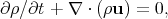 |
(7) |
 |
(8) |
where  ,
u, P
are the mass density, velocity, and pressure, and
,
u, P
are the mass density, velocity, and pressure, and
 is the shear stress tensor. The last term is often written as
(2u +
[ ⋅ u] / 3),
where ~ 1020
c5 / n is the kinematic
viscosity (in cm2 s-1) for thermal speed
c5 in units of
105 cm s-1 and density n in
cm-3. This form of
is only valid in an
incompressible fluid since the
viscosity depends on density (and temperature). The scale
LK at
which the dissipation rate equals the advection rate is called the
Kolmogorov microscale and is approximately
LK = 1015 / (nMa) cm.
is the shear stress tensor. The last term is often written as
(2u +
[ ⋅ u] / 3),
where ~ 1020
c5 / n is the kinematic
viscosity (in cm2 s-1) for thermal speed
c5 in units of
105 cm s-1 and density n in
cm-3. This form of
is only valid in an
incompressible fluid since the
viscosity depends on density (and temperature). The scale
LK at
which the dissipation rate equals the advection rate is called the
Kolmogorov microscale and is approximately
LK = 1015 / (nMa) cm.
In the compressible case, the scale at which dissipation dominates
advection will vary with position because of the large density
variations. This could spread out the region in wave number space
at which any power-law cascade steepens into the dissipation
range. Usually the viscosity is assumed to be constant for ISM
turbulence. The force per unit mass F may include
self-gravity and magnetism, which introduce other equations to be
solved, such as the Poisson and induction equations. The pressure
P is related to the other variables through the internal energy
equation. For this discussion, we assume an isentropic (or
barotropic) equation of state, P ~
 , with
a
parameter (= 1 for an isothermal gas). The inclusion of an
energy equation is crucial for ISM turbulence; otherwise the
energy transfer between kinetic and thermal modes may be
incorrect. An important dimensionless number is the sonic Mach
number Ma = u / a, where a is the
sound speed. For most ISM
turbulence, Ma ~ 0.1 - 10, so it is rarely
incompressible and often supersonic, producing shocks.
, with
a
parameter (= 1 for an isothermal gas). The inclusion of an
energy equation is crucial for ISM turbulence; otherwise the
energy transfer between kinetic and thermal modes may be
incorrect. An important dimensionless number is the sonic Mach
number Ma = u / a, where a is the
sound speed. For most ISM
turbulence, Ma ~ 0.1 - 10, so it is rarely
incompressible and often supersonic, producing shocks.
4.3. Statistical Closure Theories
In turbulent flows all of the variables in the hydrodynamic equations are strongly fluctuating and can be described only statistically. The traditional practice in incompressible turbulence is to derive equations for the two- and three-point correlations as well as various other ensemble averages. An equation for the three-point correlations generates terms involving four-point correlations, and so on. The existence of unknown high-order correlations is a classical closure problem, and there are a large number of attempts to close the equations, i.e., to express the high-order correlations in terms of the low-order correlations. Examples range from simple gradient closures for mean flow quantities to mathematically complex approaches such as the Lagrangian history Direct Interaction Approximation (DIA, see Leslie 1973), the Eddy-Damped Quasi-Normal Markovian (EDQNM) closure (see Lesieur 1990), diagrammatic perturbation closures, renormalization group closures, and others (see general references given in Section 1).
The huge number of additional unclosed terms that are generated by compressible modes and thermal modes using an energy equation (see Lele 1994) render conventional closure techniques ineffective for much of the ISM, except perhaps for extremely small Mach numbers (e.g., Bertoglio, Bataille & Marion 2001). Besides their intractability, closure techniques only give information about the correlation function or power spectrum, which yields an incomplete description because all phase information is lost and higher-order moments are not treated. An exact equation for the infinite-point correlation functional can be derived (Beran 1968) but not solved. For these reasons we do not discuss closure models here. Other theories involving scaling arguments (e.g., She & Leveque 1994), statistical mechanical formulations (e.g., Shivamoggi 1997), shell models (see Biferale 2003 for a review), and dynamical phenomenology (e.g., Leorat et al. 1990) may be more useful, along with closure techniques for the one-point pdfs, such as the mapping closure (Chen, Chen & Kraichnan 1989).
4.4. Solenoidal and Compressible Modes
For compressible flows relevant to the ISM, the Helmholtz
decomposition theorem splits the velocity field into compressible
(dilatational, longitudinal) and solenoidal (rotational, vortical)
modes uc and us, defined by
×
uc = 0 and
⋅
us = 0. In strong 3D turbulence these
components have different effects, leading to shocks and
rarefactions for uc and to vortex structures for
us. Only the compressible mode is directly coupled to
the gravitational field. The two modes are themselves coupled and
exchange energy. The coupled evolution equations for the vorticity
 =
× u and
dilatation ⋅ u
contain one asymmetry that favors transfer from solenoidal to
compressible components in the absence of viscous and pressure terms
(Vázquez-Semadeni, Passot & Pouquet 1996;
Kornreich & Scalo
2000)
and another asymmetry that transfers from compressible
to solenoidal when pressure and density gradients are not aligned,
as in an oblique shock. This term in the vorticity equation,
proportional to
P ×
(1 /
), causes
baroclinic vorticity generation. If turbulence is modeled as
barotropic or isothermal, vorticity generation is suppressed. One
or the other of these asymmetries can dominate in different parts
of the ISM (Section 5).
=
× u and
dilatation ⋅ u
contain one asymmetry that favors transfer from solenoidal to
compressible components in the absence of viscous and pressure terms
(Vázquez-Semadeni, Passot & Pouquet 1996;
Kornreich & Scalo
2000)
and another asymmetry that transfers from compressible
to solenoidal when pressure and density gradients are not aligned,
as in an oblique shock. This term in the vorticity equation,
proportional to
P ×
(1 /
), causes
baroclinic vorticity generation. If turbulence is modeled as
barotropic or isothermal, vorticity generation is suppressed. One
or the other of these asymmetries can dominate in different parts
of the ISM (Section 5).
Only the solenoidal mode exists in incompressible turbulence, so vortex models can capture much of the dynamics (Pullin & Saffman 1998). Compressible supersonic turbulence has no such conceptual simplification, because even at moderate Mach numbers there will be strong interactions with the solenoidal modes, and with the thermal modes if isothermality is not assumed.
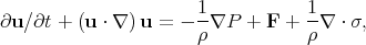
Quadratic-conserved quantities constrain the evolution of classical systems. A review of continuum systems with dual quadratic invariants is given by Hasegawa (1985). For turbulence, the important quadratic invariants are those conserved by the inviscid momentum equation. The conservation properties of turbulence differ for incompressible versus compressible, 2D versus 3D, and hydrodynamic versus MHD (see also Biskamp 2003). For incompressible flows, the momentum equation neglecting viscosity and external forces is, from Equation 8 above,
 |
(9) |
Taking the scalar product of this equation with u, integrating over all space, using Gauss' theorem, and assuming that the velocity and pressure terms vanish at infinity gives
 |
(10) |
demonstrating that kinetic energy per unit
mass is globally conserved by the advection operator. In Fourier
space this equation leads to a "detailed" conservation condition
in which only triads of wavevectors participate in energy
transfer. It is this property that makes closure descriptions in
Fourier space so valuable. Virtually all the phenomenology
associated with incompressible turbulence traces back to the
inviscid global conservation of kinetic energy; unfortunately,
compressible turbulence does not share this property. Another
quadratic conserved quantity for incompressible turbulence is
kinetic helicity <u ⋅
>, which measures the
asymmetry between vorticity and velocity fields. This is not
positive definite so its role in constraining turbulent flows is
uncertain (see
Chen, Chen & Eyink
2003).
Kurien, Taylor &
Matsumoto (2003)
find that helicity conservation controls the inertial range cascade at
large wave numbers for incompressible turbulence.
For 2D turbulence there is an additional positive-definite
quadratic invariant, the enstrophy or mean square vorticity
<( ×
u)2>. The derivative in the
enstrophy implies that it selectively decays to smaller scales
faster than the energy, with the result that the kinetic energy
undergoes an inverse cascade to smaller wave numbers. This result
was first pointed out by
Kraichnan (1967)
and has been verified in numerous experiments and simulations (see
Tabeling 2002
for a comprehensive review of 2D turbulence). Because of the absence of
the vorticity stretching term
⋅
u in the 2D
vorticity equation, which produces the complex system of vortex
worms seen in 3D turbulence, 2D turbulence evolves into a system
of vortices that grow with time through their merging.
In 2D-compressible turbulence the square of the potential
vorticity ( /
) is also
conserved
(Passot, Pouquet &
Woodward 1988),
unlike the case in 3D-compressible turbulence.
This means that results obtained from 2D simulations may not apply
to 3D. However, if energy is fed into galactic turbulence at very
large scales, e.g., by galactic rotation, then the ISM may
possesses quasi-2D structure on these scales.
Compressibility alters the conservation properties of the flow.
Momentum density
u is
the only quadratic-conserved
quantity but it is not positive definite. Momentum conservation
controls the properties of shocks in isothermal supersonic
nonmagnetic turbulence. Interacting oblique shocks generate flows
that create shocks on smaller scales
(Mac Low & Norman
1993),
possibly leading to a shock cascade controlled by momentum
conservation. Kinetic energy conservation is lost because it can
be exchanged with the thermal energy mode: compression and shocks
heat the gas. The absence of kinetic energy conservation means
that in Fourier space the property of detailed conservation by
triads is lost, and so is the basis for many varieties of
statistical closures. Energy can also be transferred between
solenoidal and compressional modes, and even when expanded to only
second order in fluctuation amplitude, combinations of any two of
the vorticity, acoustic, and entropy modes, or their
self-interactions, generate other modes.
The assumption of isothermal or isentropic flow forces a helicity conservation that is unphysical in general compressible flows; it suppresses baroclinic vorticity creation, and affects the exchange between compressible kinetic and thermal modes. Isothermality is likely to be valid in the ISM only over a narrow range of densities, from 103 to 104 cm-3 in molecular clouds for example (Scalo et al. 1998), and this is much smaller than the density variation found in simulations. Isothermality also suppresses the ability of sound waves to steepen into shocks.
Magnetic fields further complicate the situation. Energy can be
transferred between kinetic and magnetic energy so only the total,
u2 + B2 /
8 , is
conserved. Kolmogorov-type
scaling may still result in the cross-field direction
(Goldreich &
Sridhar 1995).
The magnetic helicity A ⋅ B
(A = magnetic vector potential) and cross helicity u
⋅ B are conserved but their role in the dynamics is uncertain.
Pouquet et al. (1976)
addressed the MHD energy cascade using EDQNM closure and predicted an
inverse cascade for large magnetic helicities.
Ayyer & Verma (2003)
assumed a Kolmogorov
power spectrum and found that the cascade direction depends on
whether kinetic and magnetic helicities are nonzero. Without
helicity, all the self- and cross-energy transfer between kinetic
and magnetic energies are direct, meaning to larger wave numbers,
whereas the magnetic and kinetic helical contributions give an
inverse cascade for the four sets of possible magnetic and kinetic
energy exchanges, confirming the result of
Pouquet et al. (1976).
With or without helicity, the net energy transfer within a given
wave number band is from magnetic to kinetic on average. It is
seen that while kinetic helicity cannot reverse the direct cascade
in hydrodynamic turbulence, magnetic helicity in MHD turbulence
can. The effects of kinetic and magnetic helicity on supersonic
hydrodynamic or MHD turbulence are unexplored.
, is
conserved. Kolmogorov-type
scaling may still result in the cross-field direction
(Goldreich &
Sridhar 1995).
The magnetic helicity A ⋅ B
(A = magnetic vector potential) and cross helicity u
⋅ B are conserved but their role in the dynamics is uncertain.
Pouquet et al. (1976)
addressed the MHD energy cascade using EDQNM closure and predicted an
inverse cascade for large magnetic helicities.
Ayyer & Verma (2003)
assumed a Kolmogorov
power spectrum and found that the cascade direction depends on
whether kinetic and magnetic helicities are nonzero. Without
helicity, all the self- and cross-energy transfer between kinetic
and magnetic energies are direct, meaning to larger wave numbers,
whereas the magnetic and kinetic helical contributions give an
inverse cascade for the four sets of possible magnetic and kinetic
energy exchanges, confirming the result of
Pouquet et al. (1976).
With or without helicity, the net energy transfer within a given
wave number band is from magnetic to kinetic on average. It is
seen that while kinetic helicity cannot reverse the direct cascade
in hydrodynamic turbulence, magnetic helicity in MHD turbulence
can. The effects of kinetic and magnetic helicity on supersonic
hydrodynamic or MHD turbulence are unexplored.
These considerations suggest that the type of cascade expected for highly compressible MHD turbulence in the ISM cannot be predicted yet. Numerical simulations may result in an incorrect picture of the cascade if restricted assumptions like isothermality and constant kinematic viscosity are imposed.
4.6. Scale-invariant Kinetic Energy Flux and Scaling Arguments for the Power Spectrum
In the
Kolmogorov (1941)
model of turbulence energy injected at
large scales "cascades" to smaller scales by
kinetic-energy-conserving interactions that are local in Fourier
space at a rate independent of scale, and then dissipates by
viscosity at a much smaller scale. At a given scale
 having velocity
u, the rate of change of kinetic energy per unit
mass from exchanges with other scales is
u2
divided by the characteristic timescale, taken to be
/
u.
The constant energy rate with scale gives
u ~
1/3. If one
considers u
to represent the ensemble average velocity difference over separation
, this result gives the
second-order structure function
S2() ~
2/3. In
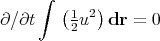
terms of wave number, uk2 ~
k-2/3, so the kinetic energy
per unit mass per unit wave number, which is the energy spectrum
E(k) (equal to
4 k2
P(k) where P(k) is the 3D power spectrum),
is given by
having velocity
u, the rate of change of kinetic energy per unit
mass from exchanges with other scales is
u2
divided by the characteristic timescale, taken to be
/
u.
The constant energy rate with scale gives
u ~
1/3. If one
considers u
to represent the ensemble average velocity difference over separation
, this result gives the
second-order structure function
S2() ~
2/3. In
terms of wave number, uk2 ~
k-2/3, so the kinetic energy
per unit mass per unit wave number, which is the energy spectrum
E(k) (equal to
4 k2
P(k) where P(k) is the 3D power spectrum),
is given by
 |
(11) |
This 5/3 law was first confirmed experimentally 20 years after Kolmogorov's proposal using tidal channel data to obtain a large inertial range (Grant, Stewart & Moillet 1962). More recent confirmations of this relation and the associated second-order structure function have used wind tunnels, jets, and counter-rotating cylinders (see Frisch 1995). The largest 3D incompressible simulations (Kaneda et al. 2003) indicate that the power-law slope of the energy spectrum might be steeper by about 0.1. Similar considerations applied to the helicity cascade (Kurien et al. 2003) predict a transition to E(k) ~ k-4/3 at large k, perhaps explaining the flattening of the spectrum, or "bottleneck effect" seen in many simulations. Leorat, Passot & Pouquet (1990) generalized the energy cascade phenomenology to the compressible case assuming locality of energy transfer (no shocks), but allowing for the fact that the kinetic energy transfer rate will not be constant. It is commonly supposed that highly supersonic turbulence should have the spectrum of a field of uncorrelated shocks, k-2 (Saffman 1971), although this result has never been derived in more than one-dimension, and shocks in most turbulence should be correlated.
These scaling arguments make only a weak connection with the hydrodynamical equations, either through a conservation property or an assumed geometry (see also Section 4.1). The only derivation of the -5/3 spectrum for incompressible turbulence that is based on an approximate solution of the Navier-Stokes equation is Lundgren's (1982) analysis of an unsteady stretched-spiral vortex model for the fine-scale structure (see Pullin & Saffman 1998). No such derivation exists for compressible turbulence.
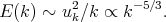
Kolmogorov's (1941)
most general result is the "four-fifths
law." For statistical homogeneity, isotropy, and a stationary
state driven at large scales, the energy flux through a given
wave number band k should be independent of k for
incompressible turbulence
(Frisch 1995,
Section 6.2.4). Combined with
a rigorous relation between energy flux and the third-order
structure function, this gives
(Frisch 1995)
an exact result in the limit of small
 r:
r:
 |
(12) |
 is
the rate of dissipation due to viscosity,
v(r,
r) is the velocity difference over spatial lag
r
at position r, and the ensemble average is over all positions.
Kolmogorov (1941)
obtained this result for decaying turbulence
using simpler arguments. Notice that self-similarity is not
assumed. A more general version of this relation has been
experimentally tested by
Moisy, Tabeling, &
Willaime (1999)
and found to agree to within a few percent over a range of scales up
to three decades.
is
the rate of dissipation due to viscosity,
v(r,
r) is the velocity difference over spatial lag
r
at position r, and the ensemble average is over all positions.
Kolmogorov (1941)
obtained this result for decaying turbulence
using simpler arguments. Notice that self-similarity is not
assumed. A more general version of this relation has been
experimentally tested by
Moisy, Tabeling, &
Willaime (1999)
and found to agree to within a few percent over a range of scales up
to three decades.
For compressible ISM turbulence, kinetic energy is not conserved between scales; for this reason, the term "inertial range" is meaningless. As a result, there is no guarantee of scale-free or self-similar power-law behavior. The driving agents span a wide range of scales (Section 3) and the ISM is larger than all of them. Excitations may spread to both large and small scales, independent of the direction of net energy transfer. In the main disks of galaxies where the Toomre parameter Q is less than ~ 2, vortices larger than the disk thickness may result from quasi-2D turbulence; recall that Q equals the ratio of the scale height to the epicyclic length. Large-scale vortical motions in a compressible, self-gravitating ISM may amplify to look like flocculent spirals.
4.7. Intermittency and Structure Function Scaling
Kolmogorov's (1941)
theory did not recognize that dissipation in
turbulence is "intermittent" at small scales, with intense
regions of small filling factor, giving fat, nearly exponential
tails in the velocity difference or other probability distribution
functions (pdfs). Intermittency can refer to either the time,
space, or probability structures that arise. The best-studied
manifestation is "anomalous scaling" of the high-order velocity
structure functions (Equation 1),
S(
r) = (v[r] - v[r +
r])p
~
r p. For
Kolmogorov turbulence with the four-fifths law and an additional
assumption of self-similarity
(v(
r) = h
v( r) for small
r with
h = 1/3)
p =
p/3. In real incompressible turbulence,
p rises
more slowly with p (compare Section 4.13; e.g.,
Anselmet et al. 1984).
p. For
Kolmogorov turbulence with the four-fifths law and an additional
assumption of self-similarity
(v(
r) = h
v( r) for small
r with
h = 1/3)
p =
p/3. In real incompressible turbulence,
p rises
more slowly with p (compare Section 4.13; e.g.,
Anselmet et al. 1984).
Interstellar turbulence is probably intermittent, as indicated by the small filling fraction of clouds and their relatively high energy dissipation rates (Section 3). Velocity pdfs and velocity difference pdfs also have fat tails (Section 2), as may elemental abundance distributions (Interstellar Turbulence II). Other evidence for intermittency in the dissipation field is the 103 K collisionally excited gas required to explain CH+, HCO+, OH, and excited H2 rotational lines (Falgarone et al. 2004; Interstellar Turbulence II). Although it is difficult to distinguish between the possible dissipation mechanisms (Pety & Falgarone 2000), the dissipation regions occupy only ~ 1% of the line of sight and they seem to be ubiquitous (Falgarone et al. 2004). If they are viscous shear layers, then their sizes (1015 cm) cannot be resolved with present-day simulations.
A geometrical model for
p in
incompressible nonmagnetic turbulence was proposed by She & Leveque
(1994,
see also
Liu & She 2003).
The model considers a box of turbulent fluid
hierarchically divided into sub-boxes in which the energy
dissipation is either large or small. The mean energy flux is
conserved at all levels with Kolmogorov scaling, and the
dissipation regions are assumed to be one-dimensional vortex tubes
or worms, known from earlier experiments and simulations. Then
p was derived
to be p/9 + 2(1 - [2/3]p/3) and shown to
match the experiments up to at least p = 10 (see
Dubrulle 1994
and
Boldyrev 2002
for derivations).
Porter, Pouquet &
Woodward (2002)
found a flow dominated by vortex tubes in simulations of decaying
transonic turbulence at fairly small Mach numbers
(Figure 3) and got good agreement with the
She-Leveque
formula. A possible problem with the She-Leveque approach is that
the dimension of the most intense vorticity structures does not
have a single value, and the average value is larger than unity
for incompressible turbulence
(Vainshtein 2003).
A derivation of
p based on a
dynamical vortex model has been given by
Hatakeyama & Kambe
(1997).
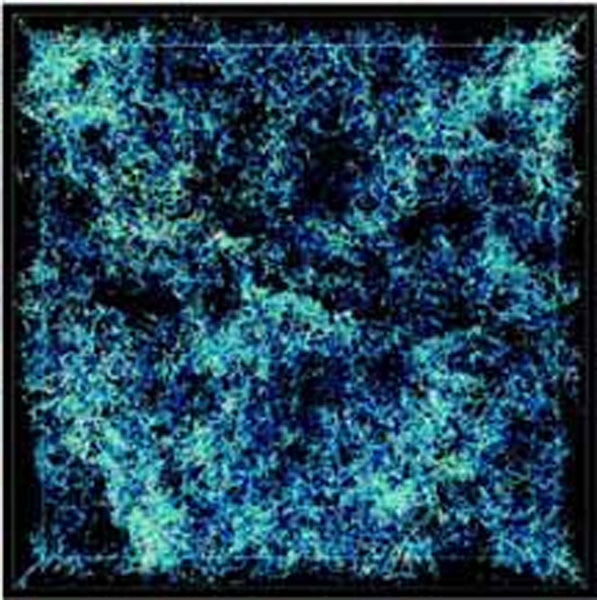 |
Figure 3. Vorticity structures in a 1024 × 1024 × 128 section of a 10243 simulation of compressible decaying nonmagnetic turbulence with initial rms Mach number of unity. From Porter, Woodward & Pouquet (1998). |
Politano & Pouquet
(1995)
proposed a generalization for the MHD
case (see also 4.13). It depends on the scaling
relations for the velocity and cascade rate, and on the
dimensionality of the dissipative structures. They noted solar
wind observations that suggested the most dissipative structures
are two dimensional current sheets.
Müller &
Biskamp (2000)
confirmed that dissipation in incompressible MHD turbulence occurs
in 2D structures, in which case
p = p/9
+ 1 - (1/3)p/3. However,
Cho, Lazarian &
Vishniac (2002a)
found that for
anisotropic incompressible MHD turbulence measured with respect to
the local field, She-Leveque scaling with 1D intermittent
structures occurs for the velocity and a slightly different
scaling occurs for the field.
Boldyrev (2002)
assumed that turbulence is mostly solenoidal with Kolmogorov scaling,
while the most dissipative structures are shocks, again getting
p =
p/9 + 1 - (1/3)p/3 because of the planar geometry; the
predicted energy spectrum was E(k) ~
k-1-2 ~
k-1.74. Boldyrev noted that the spectrum will be
steeper if the shocks have a dimension equal to the fractal dimension of
the density.
The uncertainties in measuring ISM velocities preclude a test of these relations, although they can be compared with numerical simulations. Boldyrev, Nordlund & Padoan (2002b) found good agreement in 3D super-Alfvénic isothermal simulations for both the structure functions to high order and the power spectrum. The simulations were forced solenoidally at large scales and have mostly solenoidal energy, so they satisfy the assumptions in Boldyrev (2002). Padoan et al. (2003b) showed that the dimension of the most dissipative structures varies with Mach number from one for lines at subsonic turbulence to two for sheets at Mach 10. The low Mach number result is consistent with the nonmagnetic transonic simulation in Porter et al. (2002; see Figure 3). Kritsuk & Norman (2004) showed how nonisothermality leads to more complex folded structures with dimensions larger than two.
4.8. Details of the Energy Cascade: Isotropy and Independence of Large and Small Scales
Kolmogorov's model implies an independence between large and small
scales and a resulting isotropy on the smallest scales. Various
types of evidence for and against this prediction were summarized by
Yeung & Brasseur
(1991).
One clue comes from the
incompressible Navier-Stokes equation written in terms of the
Fourier-transformed velocity. Global kinetic energy conservation
is then seen to occur only for interactions between triads of
wavevectors (e.g., Section 4.12). The trace of
the equation for the energy spectrum tensor gives the rate of
change of energy per unit wave number in Fourier modes E(k)
owing to the exchange of energy with all other modes T(k) and
the loss from viscous dissipation:
 E(k) /
t =
T(k) - 2
k2 E(k). The details of the
energy transfer can be studied by decomposing the transfer
function T(k) into a sum of contributions T(k|
p,q) defined as
the energy transfer to k resulting from interactions between
wave numbers p and q.
E(k) /
t =
T(k) - 2
k2 E(k). The details of the
energy transfer can be studied by decomposing the transfer
function T(k) into a sum of contributions T(k|
p,q) defined as
the energy transfer to k resulting from interactions between
wave numbers p and q.
Domaradzki & Rogallo (1990) and Yeung & Brasseur (1991) analyzed T(k| p, q) from simulations to show that, whereas there is a net local transfer to higher wave numbers, at smaller and smaller scales the cascade becomes progressively dominated by nonlocal triads in which one leg is in the energy-containing (low-k) range. This means that small scales are not decoupled from large scales. Waleffe (1992) pointed out that highly nonlocal triad groups tend to cancel each other in the net energy transfer for isotropic turbulence; the greatest contribution is from triads with a scale disparity of about an order of magnitude (Zhou 1993). Yeung & Brasseur (1991) and Zhou, Yeung & Brasseur (1996) demonstrated that long-range couplings are important in causing small-scale anisotropy in response to large-scale anisotropic forcing, and that this effect increases with Reynolds number.
The kinetic energy transfer between scales can be much more complex in the highly compressible case where the utility of triad interactions is lost. Fluctuations with any number of wavevector combinations can contribute to the energy transfer. Momentum density is still conserved in triads, but the consequences of this are unknown. Even in the case of very weakly compressible turbulence, Bataille & Zhou (1999) found 17 separate contributions to the total compressible transfer function T(k). Nevertheless, the EDQNM closure theory applied to very weakly compressible turbulence by Bataille & Zhou (1999) and Bertoglio, Bataille & Marion (2001), assuming only triadic interactions, yields interesting results that may be relevant to warm H I, the hot ionized ISM, or dense molecular cores where the turbulent Mach number might be small. Then the dominant compressible energy transfer is not cascade-type but a cross-transfer involving local (in spectral space) transfer from solenoidal to compressible energy. At Mach numbers approaching unity (for which the theory is not really valid) the transfer changes to cascade-type, with a net flux to higher wave numbers.
Pouquet et al. (1976) were among the first to address the locality and direction of the MHD energy cascade using a closure method. For more discussions see Ayyer & Verma (2003), Biferale (2003) and Biskamp (2003).
4.9. Velocity Probability Distribution
A large number of papers have demonstrated non-Gaussian behavior
in the pdfs of vorticity, energy dissipation, passive scalars, and
fluctuations in the pressure and nonlinear advection, all for
incompressible turbulence. Often the pdfs have excess tails that
tend toward exponentials at small scale (see
Chen et al. 1989;
Castaing, Gagne &
Hopfinger 1990
for early references). Velocity fluctuation differences and derivatives
exhibit tails of the form
exp(-v )
with 1 < < 2 and
~ 1 at small scale (e.g.,
Anselmet et al. 1984,
She et al. 1993).
Physically this is a manifestation of intermittency, with the most
intense turbulence becoming less space-filling at smaller scales.
The behavior may result from the stretching properties of the
advection operator (see
She 1991
for a review).
)
with 1 < < 2 and
~ 1 at small scale (e.g.,
Anselmet et al. 1984,
She et al. 1993).
Physically this is a manifestation of intermittency, with the most
intense turbulence becoming less space-filling at smaller scales.
The behavior may result from the stretching properties of the
advection operator (see
She 1991
for a review).
This same kind of behavior has been observed for the ISM in the form of excess CO line wings (Falgarone & Phillips 1990) and in the pdfs of CO (Padoan et al. 1997, Lis et al. 1998, Miesch et al. 1999) and H I (Miville-Deschênes, Joncas & Falgarone 1999) centroid velocities. The regions include quiescent and active star formation, diffuse H I, and self-gravitating molecular clouds. Lis et al. (1996, 1998) compared the observations with simulations of mildly supersonic decaying turbulence and associated the velocity-difference pdf tails with filamentary structures and regions of large vorticity.
The first comparison of observations with simulations for velocity difference pdfs was given by Falgarone et al. (1994), who used optically thin line profile shapes from a simulation of decaying transonic hydrodynamic turbulence. They found that the excess wings could be identified in some cases with localized regions of intense vorticity. Klessen (2000) compared observations with the centroid-velocity-difference distributions from isothermal hydrodynamic simulations and found fair agreement with an approach to exponential tails on the smallest scales. Smith, Mac Low & Zuev (2000) found an exponential distribution of velocity differences across shocks in simulations of hypersonic decaying turbulence and were able to derive this result using an extension of the mapping closure technique (e.g., Gotoh & Kraichnan 1993). Ossenkopf & Mac Low (2002) gave a detailed comparison between observations of the Polaris flare and MHD simulation velocity and velocity centroid-difference pdfs, along with other descriptors of the velocity field. Cosmological-scale galaxy velocity-difference pdfs (Seto & Yokoyama 1998) also exhibit exponential forms at small separations.
The pdf of the velocity itself is not yet understood. The argument that the velocity pdf should be Gaussian based on the central-limit theorem applied to independent Fourier coefficients of an expansion of the velocity field, or to sums of independent velocity changes (e.g., Tennekes & Lumley 1972), neglects correlations and only applies to velocities within a few standard deviations of the mean. Perhaps this is why the early work found Gaussian velocity pdfs (e.g., Monin & Yaglom 1975, Kida & Murakami 1989, Figure 6; Jayesh & Warhaft 1991, Figure 1; Chen et al. 1993, Figure 3). The velocity pdf must possess nonzero skewness (unlike a Gaussian) in order to have energy transfer among scales (e.g., Lesieur 1990).
Recent evidence for non-Gaussian velocity pdfs have been found for incompressible turbulence from experimental atmospheric data (Sreenivasan & Dhruva 1998), turbulent jets (Noullez et al. 1997), boundary layers (Mouri et al. 2003), and quasi-2D turbulence (Bracco et al. 2000). The sub-Gaussian results (with pdf flatness factor F = < u4 > / < u2 > less than 3) are probably from the dominance of a small number of large-scale modes, while the hyper-Gaussian results (F > 3) may be the result of correlations between Fourier modes Mouri et al. 2003), an alignment of vortex tubes (Takaoka 1995), or intermittency (Schlichting & Gersten 2000). The results are unexplained quantitatively.
For the ISM, exponential or 1/v centroid-velocity distributions were discovered and rediscovered several times over the past few decades (see Miesch, Scalo & Bally 1999). Miesch & Scalo (1995) and Miesch et al. (1999) found near-exponential tails in the 13CO centroid-velocity pdfs of several molecular regions. The pdf of the H I gas centroid-velocity component perpendicular to the disk of the LMC is also an exponential (Kim et al. 1998).
Rigorous derivations of the equation for the velocity pdf of incompressible hydrodynamic turbulence are presented in Chapter 12 and Appendix H of Pope (2000). Dopazo, Valino & Fueyo (1997) show how to derive evolution equations for the moments of the velocity distribution from the kinetic equation. Closure methods for pdf equations are discussed in Chen & Kollman (1994), Dopazo (1994), Dopazo et al. (1997), and Pope (2000). Results generally predict Gaussian pdfs, although this depends somewhat on the closure method and assumptions.
Simulations have not generally examined the velocity pdf in detail, and when they have, the centroid-velocity pdf or optically thin line profile is usually given. An important exception is the 3D incompressible simulation of homogeneous shear flows by Pumir (1996), who found nearly exponential velocity fluctuation pdfs for velocity components perpendicular to the streamwise component. However, for conditions more applicable to the compressible ISM, the results are mixed. Smith, Mac Low & Zuev (2000) found a Gaussian distribution of shock speeds in 3D simulations of hypersonic decaying turbulence, but did not relate this to the pdf of the total velocity field. Lis et al. (1996) found the pdf of centroid velocities to be Gaussian or sub-Gaussian in hydrodynamic simulations of transonic compressible turbulence. The centroid velocity pdf for a 3D-forced MHD simulation given by Padoan et al. (1999) looks Gaussian at velocities above the mean but has a fat tail at small velocities. A detailed simulation study of the centroid-velocity pdf was presented by Klessen (2000), who examined driven and decaying hydrodynamic simulations with and without self-gravity at various Mach numbers. The centroid pdfs are nearly Gaussian, but the 3D pdfs were not discussed. The only 3D (not centroid) velocity pdf for an ISM-like simulation we know of, a decaying MHD simulation with initial Mach number of 5 displayed by Ossenkopf & Mac Low (2002, Figure 11a), is distinctly exponential deep into the pdf core at their highest resolution run; nevertheless they remark in the text that all the pdfs are Gaussian.
Chappell & Scalo (2001) found nearly-exponential tails in 2D simulations of wind-driven pressureless (Burgers) turbulence, and showed that the tail excesses persisted even in the absence of forcing. They proposed that these excesses could be understood in terms of the extreme inelasticity of the shell interactions in the Burgers model, and speculated that the result could be more general for systems in which interactions are inelastic, so that kinetic energy is not a globally conserved quantity. For example, a Gibbs ensemble for particles that conserve mass and momentum, but not energy, gives an exponential velocity distribution. Ricotti & Ferrara (2002) studied simulated systems of inelastically colliding clouds driven by supernovae and showed how the velocity pdf of the clouds approaches an exponential as the assumed inelasticity becomes large. Hyper-Gaussian velocity distributions with exponential and even algebraic tails have also been observed in laboratory and simulated inelastic granular fluids (Barrat & Trizac 2002, Ben-Naim & Krapivsky 2002, Radjai & Roux 2002). All of these systems dissipate energy on all scales.
The reason for the fat tails may be the positive velocity fluctuation correlations introduced by the inelasticity. This can be seen by noting that successive velocities are positively correlated for inelastic point particles conserving mass and momentum but not energy. Then the velocity changes are not independent and the central limit theorem does not apply (see Mouri et al. 2003). Such correlations, resulting entirely from the large range of dissipation scales, would be a fundamental difference between incompressible and supersonic turbulence. If true, then hyper-Gaussian pdfs need not be a signature of intermittency (Klessen 2000).
The idea of turbulent "pressure" is difficult to avoid because of its convenience. It has been used to generalize the gravitational instability (e.g., Bonazzola et al. 1987, Vázquez-Semadeni & Gazol 1995), to confine molecular clouds (e.g., McKee & Zweibel 1992, Zweibel & McKee 1995), and to approximate an equation of state (e.g., Vázquez-Semadeni, Canto & Lizano 1998). Rigorous analysis (Bonazzola et al. 1992) shows that turbulence can be represented as a pressure only if the dominant scale is much smaller than the size of the region under consideration ("microturbulence"). In fact this is not the case. The turbulent energy spectrum places most of the energy on the largest scale, and because the spectrum is continuous, the scale separation required for the definition of pressure (Bonazzola et al. 1992) does not exist. Ballesteros-Paredes, Vázquez-Semadeni & Scalo (1999) evaluated the volume and surface terms in the virial theorem and showed that the kinetic energy surface term is so large that the main effect of turbulence is to distort, form, and dissolve clouds rather than maintain them as quasi-permanent entities. Supersonic turbulence is also likely to be dominated by highly intermittent shocks whose effect is difficult to model as a pressure even with an ensemble average.
Simulations of turbulent fragmentation in self-gravitating clouds show that turbulence suppresses global collapse while local collapse occurs in cores produced by the turbulence (Sections 5.10 and 5.11). This process does not resemble pressure, however. Global collapse is avoided because the gravitational and turbulent energies are transferred to separate pieces that have smaller and smaller scales.
4.11. Below the Collision Mean Free Path
Scintillation observations suggest interstellar electron density irregularities extend at a weak level down to tens or hundreds of kilometers Interstellar Turbulence II), which is slightly larger than the ion gyroradius (mi cvth / eB ~ 108 / B(µ G) cm) in the warm ionized medium and much smaller than the ion-neutral (1015 / n cm) and Coulomb (1014 / ni cm) mean free paths at unit density, n and ni. Collisionless plasma processes involving magnetic irregularities on small scales are probably involved.
Collisionless plasmas behave like a fluid on scales larger than the ion cyclotron radius. The equation of motion includes the coupling between charged particles and the magnetic field. There are also equations for mass and magnetic flux continuity and for the heat flux. The parallel and perpendicular components of the pressure tensor that account for their gyromotions were included by Chew, Goldberger & Low (1956). A general review is in Kulsrud (1983). Dissipation on very small scales is by cyclotron resonance, which is not considered in these equations. Dissipation on scales larger than the cyclotron radius is by Landau damping and other processes, such as Ohmic and ambipolar diffusion. Landau damping arises from a resonance between particle thermal speeds and wave speeds in various directions. Proper treatment of Landau damping in ISM turbulence is essential for understanding fast mode waves that may scatter cosmic rays (Interstellar Turbulence II). Landau damping could also modify the energy cascade because it covers a wide range of scales.
Landau damping was included in the MHD equations by
Snyder, Hammett &
Dorland (1997).
Passot & Sulem
(2003a)
added dispersive effects that are important on scales close to the ion
inertial length, vA /
 i, for
Alfvén speed vA = B /
(4
)1/2 and
cyclotron frequency
i =
eB / mc. They used the equations of
continuity and motion plus Ohm's law for the time derivative of the
perturbed field b:
i, for
Alfvén speed vA = B /
(4
)1/2 and
cyclotron frequency
i =
eB / mc. They used the equations of
continuity and motion plus Ohm's law for the time derivative of the
perturbed field b:
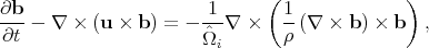 |
(13) |
where the quantities
are normalized to the ambient field and Alfvén speed, and
 i =
i
L / vA is the normalized ion cyclotron
frequency for system scale L. The last term is the Hall term,
which comes from the inertia of the ions as the magnetic field
follows the electrons. Pressure and density can be related by an
equation for the heat flux
(Passot & Sulem
2003a)
or an adiabatic power law on scales larger than the mean free path
(Laveder, Passot &
Sulem 2001).
The result is a system of equations for
Hall-MHD. An interesting instability appears in this regime
resulting in a collapse of gas and field into thin helical filaments
(Laveder, Passot &
Sulem 2001,
2002).
Because the instability still operates in the collisionless regime
(Passot & Sulem
2003b),
such filaments may account for some of the elongated
structure seen by ISM scintillation on scales smaller than the
collision mean free path.
i =
i
L / vA is the normalized ion cyclotron
frequency for system scale L. The last term is the Hall term,
which comes from the inertia of the ions as the magnetic field
follows the electrons. Pressure and density can be related by an
equation for the heat flux
(Passot & Sulem
2003a)
or an adiabatic power law on scales larger than the mean free path
(Laveder, Passot &
Sulem 2001).
The result is a system of equations for
Hall-MHD. An interesting instability appears in this regime
resulting in a collapse of gas and field into thin helical filaments
(Laveder, Passot &
Sulem 2001,
2002).
Because the instability still operates in the collisionless regime
(Passot & Sulem
2003b),
such filaments may account for some of the elongated
structure seen by ISM scintillation on scales smaller than the
collision mean free path.
4.12. MHD Turbulence Theory: Power Spectra
The hydrodynamic turbulent cascades and intermittency effects discussed in Sections 4.6 and 4.7 have analogs in the magnetohydrodynamic case. An important difference between MHD and hydrodynamic turbulence arises because the magnetic field gives a preferred direction for forces. Turbulence in the solar wind (Matthaeus, Bieber & Zank 1995) and on the scale of interstellar scintillations is anisotropic with larger gradients of density perpendicular to the field. Shebalin et al. (1983) showed from incompressible numerical simulations with a background magnetic field that the energy spectrum of velocity fluctuations parallel to the field is steeper than perpendicular, which suggests a diminished cascade in the parallel direction and increasing anisotropy on small scales. The suppression of the parallel cascade depends on the strength of the mean field, increasing for stronger fields (Müller, Biskamp & Grappin 2003). In the extreme case, there is no cascade at all in the parallel direction, leading to purely 2D or quasi-2D turbulence (Zank & Matthaeus 1993, Chen & Kraichnan 1997, Matthaeus et al. 1998). Parallel structures at high spatial frequencies passively follow the longer wavelengths in incompressible MHD without cascading to the dissipation range (Kinney & McWilliams 1998).
Incompressible MHD turbulence can be characterized in terms of
interactions between three shear-Alfvén wave packets
(Montgomery &
Matthaeus 1995,
Ng & Bhattacharjee
1996,
Galtier et al. 2000),
which satisfy the wave number and frequency sum conditions,
k1 + k2 = k3 and
1 +
2 =
3, to
conserve momentum and energy. When the interacting waves are
Alfvén waves, =
k||
va, and when they are oppositely
directed, k1 and k2 have opposite signs.
Then solutions exist only when the parallel Fourier modes have
energy at k1|| = 0 or k2|| = 0,
which correspond to long-wavelength field-line wandering. Also, when
k|| = 0, there is no cascade in the parallel direction
(e.g.,
Bhattacharjee & Ng
2001,
Galtier et al. 2002).
In this limit of incompressible or
weakly compressible MHD with a strong mean field, the transverse
velocity scales with wave number as
v
 k-1/2 and the 1D transverse energy scales as
E(k)
k-2
(Ng &
Bhattacharjee 1997,
Goldreich &
Sridhar 1997,
Galtier et al. 2000).
k-1/2 and the 1D transverse energy scales as
E(k)
k-2
(Ng &
Bhattacharjee 1997,
Goldreich &
Sridhar 1997,
Galtier et al. 2000).
Velocity and energy scalings with wave number may be obtained
from heuristic arguments that give physical insight to turbulence
theory
(Connaughton, Nazarenko
& Newell 2003).
There are two important rates, the eddy interaction rate,
int, and
the cascade rate,
cas. These
rates are related by the
number N of interactions the fluid has to experience before the
energy at a certain wave number cascades,
cas =
int /
N. For weak interactions, the velocity
change per interaction,
v, is small and
the number required is determined by a random walk: N ~ (v /
v)2.
For strong interactions, each one is significant, so
v ~ v and
N ~ 1. The velocity change comes
from the integral over the equation of motion for an interaction time:
v = (dv /
dt)
int-1. The most important
acceleration is the inertial term, v ⋅
v,
giving dv/dt ~ kv2 for wave number
k and velocity v in the cascading direction.
When v has this
form, the interaction may be viewed as
consisting of three waves; three-wave systems have a constant
flux of energy, which is the cascade over wave number
(Zakharov, L'vov & Falkovich 1992).
Some systems such as gravity waves in deep water
(Pushkarev, Resio,
Zakharov 2003)
have stronger four-wave
interactions, and these conserve both energy and wave-action.
Their velocity change is given by
v =
(d2 v / dt2)
int-2.
The last step in the derivation of the energy spectrum for weak
turbulence is to assume a constant energy flux in wave number
space, where energy is the square of the perturbed velocity or the
summed squares of the velocity and the perturbed field:
=
v2
cas.
Combining terms for three-wave interactions, we get,
 |
(14) |
For weak nearly
incompressible turbulence the interaction consists of oppositely
directed "waves" or Fourier components moving at the Alfvén
speed. The interaction rate is
int =
k|| vA for parallel
wave number k|| and Alfvén speed
vA. When the field is
strong, k|| ~ constant so
int ~
constant, giving a transverse velocity scaling
v
k-1/2 from
equation (14). The energy spectrum follows from the relation
 E(k) dk = v2, so
that E(k)
v2
/ k
k-2. This is the result obtained by
Ng & Bhattacharjee
(1997)
and others.
E(k) dk = v2, so
that E(k)
v2
/ k
k-2. This is the result obtained by
Ng & Bhattacharjee
(1997)
and others.
The Kolmogorov spectrum follows
from an isotropic picture in which the wave number and velocity of
the incoming perturbations are the same as those leaving the
interaction as part of the cascade. Then
int =
kv and
v3k = constant, giving E(k)
k-5/3.
Goldreich &
Sridhar (1997)
proposed that weak MHD turbulence is
irrelevant in the ISM because it quickly strengthens in the
cascade. They suggested that ISM turbulence is usually strong,
and in this case there is a simplification that can be made from a
critical balance condition,
cas =
int
(Goldreich &
Sridhar 1995).
This condition gives a parallel cascade and
Kolmogorov scaling for transverse motions because if
=
v4
k2 /
cas from equation
(14) and cas =
k
v, then
the energy
flux is =
v3
k.
Goldreich & Sridhar reasoned that inequalities between
cas and
int would
lead to changes in the interaction process that would restore
equality. If
cas >
int, for
example, then local
field line curvature would decrease in time as the transverse
energy leaked away without adequate replacement from the parallel
direction. The field lines would then be more easily bent by the
next incoming packet. An important assumption for their model is
that the wave interactions that dominate the energy transfer are
local in wave number space (see
Lithwick &
Goldreich 2003).
For isotropic turbulence with a fixed incoming velocity, such as
an Alfvén speed,
int =
kvA. Then one of the k's
cancels from the numerator in Equation 14, but a
velocity does not cancel, giving v4 k =
constant and E(k)
k-3/2. This is the scaling suggested by
Iroshnikov (1964)
and
Kraichnan (1965)
for magnetic turbulence, before the anisotropy of
this turbulence was appreciated. Recent studies of 2D MHD
turbulence show Iroshnikov-Kraichnan scaling also
(Politano, Pouquet &
Carbone 1998;
Biskamp & Schwarz
2001;
Lee et al. 2003).
Politano et al. actually got
4 ~ 1, which
corresponds to < v4 >
k-1, but they got
2 ~ 0.7, which
gives about the Kolmogorov 1D energy
spectrum, k-1.7. The nonlinear dependence of
p on p
is the result of intermittency.
Iroshnikov-Kraichnan scaling and a suppressed parallel cascade occurs in incompressible MHD turbulence if the energy transfer among modes is dominated by interactions between waves with very different sizes (Nakayama 2002). It may also apply in 2D MHD turbulence with such nonlocal interactions (Pouquet, Frisch & Léorat 1976). The issue of locality in wave number space is not understood even in hydrodynamic turbulence (Yeung, Brasseur & Wang 1995) although local transfer is commonly assumed. A study of the degree of cancellation of long-range three-wave interactions in incompressible hydrodynamic turbulence by Zhou, Yeung & Brasseur (1996) shows that nonlocal interactions cause anisotropy at small scales, and the effect may increase with the scale separation. This suggests that long-range dynamics persist at large Reynolds numbers, in which case current MHD simulations may not have the resolution to capture the effect.
Kolmogorov k-5/3 scaling changes over to
Iroshnikov-Kraichnan k-3/2 scaling as the mean field
gets stronger, all else being equal.
Müller, Biskamp
& Grappin (2003)
found this from
simulations of incompressible turbulence using a spectral code of
size 5123. As the transition to k-3/2
occurred, the inertial range parallel to the mean field became shorter
indicating an inability to cascade in this direction, as mentioned above.
Dmitruk, Gómez
& Matthaeus (2003)
also found a spectral slope that depends sensitively on conditions. They
considered incompressible turbulence driven at speed
vd at two opposing
boundaries of an elongated box measuring
L ×
L ×
L||. When the ratio of the Alfvén propagation
time along the field, L|| / vA, to
the stirring time perpendicular to the field,
L /
vd, was large, the
relatively rapid stirring produced more small-scale structure and
a shallow energy spectrum. When the ratio was small, the spectrum
was steep.
The energy spectrum of weak nonmagnetic turbulence driven in a rapidly rotating medium also shows Iroshnikov-Kraichnan scaling in a direction perpendicular to the spin axis (Galtier 2003).
Scintillation observations (Interstellar Turbulence II)
suggest the energy spectrum of density fluctuations is close to
Kolmogorov. This limits the range of possible models in these
applications. Also, the relevance of scaling laws derived under
the assumption of weak turbulence (N = (v /
v)2 >> 1) is questionable. For these reasons,
there is continued interest in the critical balance model of strong
turbulence discussed by Goldreich and collaborators. We review
their proposals and the related numerical simulations next.
4.13. The Anisotropic Kolmogorov Model
Goldreich &
Sridhar (1995)
proposed that interstellar turbulence
on small scales results from nonlinear interactions between shear
Alfvén waves in an incompressible, ionized medium. The energy
spectrum was determined from a critical balance condition that the
wave interaction rate in the parallel direction,
int ~
k|| vA, is comparable to the cascade
rate in the perpendicular
direction, cas ~
k
v.
This condition gives a cascading energy flux
~
v2
cas ~
v3
k, which
leads to a scaling relation for perpendicular motions,
v /
vA ~
( /
L)1/3, and a cascade in the parallel
direction, making k|| L ~
(k
L)2/3. Here
L is the scale at which extrapolated turbulent motions would be
isotropic and comparable to the Alfvén speed, vA.
The energy spectrum is related to the velocity scaling law as
v2 =
E(k)dk.
Cho, Lazarian &
Vishniac (2002a)
found from 3D MHD simulations that the energy spectrum for
parallel motions is E(k||) ~
k||-2. They also obtained
k||
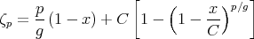
k2/3 as above and fit the 3D power spectrum
to
 |
(15) |
for unperturbed field strength B0.
In this model, perturbations get stronger as they cascade to
smaller scales, and they get more elongated with
|| /
~ (2 L /
)1/3 increasing for smaller
(|| /
~ 1000
on the smallest scales). These local relations also follow if the local
anisotropy, k|| /
k,
is proportional to the ratio of the local perturbed
field to the total field
(Matthaeus et
al. 1998;
Cho, Lazarian &
Vishniac 2003a).
The global relation between
|| and
,
averaged over a large scale, can actually be more isotropic,
~
||, if the
local field lines bend significantly on the small scale
(Cho, Lazarian &
Vishniac 2002a).
A schematic diagram of a turbulent cascade is shown in figure 4, from Maron & Goldreich (2001). Wave packets travel along the field and become distorted as the lines of force interchange with other lines containing different waves. A density pattern gets distorted by this motion too.
 |
Figure 4. (left) Distorted field lines with a downward propagating wave, and (right) distortion of a bulls-eye pattern moving upward along these lines. From Maron & Goldreich (2001). |
Electron density fluctuations in the theory of Goldreich & Sridhar (1995) are a combination of entropy fluctuations, i.e., temperature changes with approximate pressure equilibrium (Higdon 1986), and slow-mode wave compressions (Lithwick & Goldreich 2001). Turbulence distorts and divides the large-scale density structures into smaller structures, giving them the same power spectrum as the velocity. This is "passive mixing" if the density irregularities are weak and have little back reaction on the velocity field.
Passive mixing is a key component of the Goldreich et al. model
for which essentially all of the dynamics comes from
incompressible waves. Numerical simulations confirm the small
degree of coupling between these Alfvén shear modes and the
compressional modes, which are the fast and slow magnetosonic
modes (Section 4.1 in Interstellar Turbulence II).
Cho & Lazarian
(2002b)
considered the low
 =
Pthermal / Pmag
case and separated the shear, fast, and slow modes in a
compressible MHD simulation. The relative energy in the
compressible part grew from zero to only 5%-10% after three
crossing times, which implies the slow mode is weakly coupled to
the shear mode. For purely solenoidal driving, the Alfvén and
slow modes had k-5/3 energy scaling for velocity and
field, and the slow mode had k-5/3 scaling for the
density; the fast
modes had all three variables scale like k-3/2.
Cho & Lazarian
(2003)
did similar calculations for the high
case
and got the same results for mode coupling and energy spectra.
Most of the density structure was from slow modes at low
,
but at high
it came
from a nearly equal combination of slow and fast modes.
Cho & Lazarian
(2003)
showed that even for highly compressible supersonic turbulence, the
Alfvén mode, which barely couples to the compression, cascades like
an incompressible fluid with an energy spectrum
k-5/3.
=
Pthermal / Pmag
case and separated the shear, fast, and slow modes in a
compressible MHD simulation. The relative energy in the
compressible part grew from zero to only 5%-10% after three
crossing times, which implies the slow mode is weakly coupled to
the shear mode. For purely solenoidal driving, the Alfvén and
slow modes had k-5/3 energy scaling for velocity and
field, and the slow mode had k-5/3 scaling for the
density; the fast
modes had all three variables scale like k-3/2.
Cho & Lazarian
(2003)
did similar calculations for the high
case
and got the same results for mode coupling and energy spectra.
Most of the density structure was from slow modes at low
,
but at high
it came
from a nearly equal combination of slow and fast modes.
Cho & Lazarian
(2003)
showed that even for highly compressible supersonic turbulence, the
Alfvén mode, which barely couples to the compression, cascades like
an incompressible fluid with an energy spectrum
k-5/3.
These scalings are consistent with the isotropies measured for the
three modes
(Cho & Lazarian
2002b).
Alfvén modes and their
passive slow counterparts have velocities that depend on the
propagation direction relative to the field (at low
). This
makes them anisotropic with k||
k2/3, as
discussed above. Fast modes have equal velocities in all directions at low
, and the
resulting isotropy makes
k||
k, as
proposed by
Kraichnan (1965).
Cho & Lazarian
(2002b)
further reasoned that slow modes are passive at
low
because they move very slowly relative to the Alfvén
waves (a cos  << vA for thermal
speed a), so the Alfvén waves can distort them easily.
<< vA for thermal
speed a), so the Alfvén waves can distort them easily.
Cho, Lazarian &
Vishniac (2002b)
proposed that magnetic
irregularities should persist without corresponding velocity
irregularities below the viscous damping length (LK, see
Section 4.2), down to the scale at which magnetic
diffusion becomes important. Damping in the equation of motion
comes from a term
2 v,
and magnetic diffusion comes from a term like
 2
B; the ratio /
is the
Prandtl number. Cho et al. considered large Prandtl numbers and
found that the kinetic energy between the viscous and the
diffusion lengths cascaded more steeply than the magnetic energy:
Ev(k)
k-4.5 and
EB(k)
k-1. The latter relation implies that the
perturbed field,
B, is
independent of scale (using kEb(k) ~
b2), presumably because the cascade time into
the pure-magnetic regime is equal to the cascade time at its outer
scale, which is the viscous scale
(Cho, Lazarian &
Vishniac 2003b).
In their compressible MHD simulations,
Cho, Lazarian &
Vishniac (2003b)
and
Cho & Lazarian
(2003)
found density fluctuations below the viscous length with the same power
spectrum as the field,
E(k) ~ k-1. More recently,
Lazarian, Vishniac &
Cho (2004)
suggested that velocity fluctuations below the viscous length can be
driven by magnetic fluctuations.
Schekochihin et
al. (2002)
found a folded field line
structure on small scales in incompressible MHD simulations at
high Prandtl number, with the most sharply curved fields being the
weakest. They also found comparable magnetic and kinetic energy
densities and explained this result in terms of a back-reaction of
the field on the motions.
2
B; the ratio /
is the
Prandtl number. Cho et al. considered large Prandtl numbers and
found that the kinetic energy between the viscous and the
diffusion lengths cascaded more steeply than the magnetic energy:
Ev(k)
k-4.5 and
EB(k)
k-1. The latter relation implies that the
perturbed field,
B, is
independent of scale (using kEb(k) ~
b2), presumably because the cascade time into
the pure-magnetic regime is equal to the cascade time at its outer
scale, which is the viscous scale
(Cho, Lazarian &
Vishniac 2003b).
In their compressible MHD simulations,
Cho, Lazarian &
Vishniac (2003b)
and
Cho & Lazarian
(2003)
found density fluctuations below the viscous length with the same power
spectrum as the field,
E(k) ~ k-1. More recently,
Lazarian, Vishniac &
Cho (2004)
suggested that velocity fluctuations below the viscous length can be
driven by magnetic fluctuations.
Schekochihin et
al. (2002)
found a folded field line
structure on small scales in incompressible MHD simulations at
high Prandtl number, with the most sharply curved fields being the
weakest. They also found comparable magnetic and kinetic energy
densities and explained this result in terms of a back-reaction of
the field on the motions.
Maron & Goldreich (2001) and Cho, Lazarian & Vishniac (2002a) studied the velocity structure functions in strong incompressible MHD turbulence. Recall that in a power-law approximation, these functions can be written
 |
(16) |
for two points separated by distance
r. For Kolmogorov
turbulence without intermittency,
p = p /
3; with intermittency,
p(p) is
nonlinear.
Politano & Pouquet
(1995)
derived
p(p) as
 |
(17) |
where g is the exponent in the velocity relation
v
k-1/g, x is the exponent in the
cascade rate,
cas
kx, and C is the codimension of
the dissipation region: C = 2 for lines and C = 1 for
sheets (the codimension is equal to the number of spatial dimensions
minus the fractal dimension of the structure). For nonmagnetic Kolmogorov
turbulence with intermittency, g = 3, x = 2/3, and
C = 2, giving the expression for
p(p)
originally found by
She & Leveque
(1994).
Cho, Lazarian & Vishniac (2002a)
determined that strong turbulent
motions perpendicular to the local field have the same
p(p)
dependence as nonmagnetic turbulence. Relative to the
global magnetic field, the scaling of the perpendicular velocity
structure function was different
(Cho, Lazarian &
Vishniac 2003b),
following instead a form with C = 1 (sheet-like) as suggested by
Müller &
Biskamp (2000).
In both cases, the magnetic structure function had an index
p that was lower
than the velocity structure function, suggesting that
B is
more intermittent than
v.
The structure function of velocity parallel to the mean local field had
p larger than for
v
by a factor of 1.5, which is consistent with the
elongated geometry of the turbulence, for which
||3/2
(Cho, Lazarian &
Vishniac 2002a).
Haugen et al. (2003) did 10243 simulations of forced, weakly-compressible, nonhelical MHD turbulence and found a codimension of C ~ 1.8 (nearly line-like). The total energy spectrum integrated over 3D shells in k-space is ~ k-5/3 at small k and ~ k-1.5 at intermediate k just before the dissipation range. This flattening to k-1.5 was attributed to a bottleneck in the cascade and not an Iroshnikov-Kraichnan inertial spectrum. In the saturated state, 70% of the energy was kinetic but 70% of the dissipation occurred by magnetic resistivity. Such Ohmic dissipation can increase the temperature in a turbulent medium by an order of magnitude (Brandenburg et al. 1996).
Simulations of compressible MHD turbulence with zero mean field
(Cho, Lazarian &
Vishniac 2003b)
had p for velocity
the same as for incompressible turbulence, giving C = 2, and they
had p for the
field in global coordinates satisfying the
above expression with C = 1. Maps of the high-k field
structure in planes perpendicular to the mean field clearly showed this
sheet-like field geometry for both compressible and incompressible
cases. There was a transition from somewhat uniform magnetic waves
on large scales to highly intermittent sheet-like regions on small scales.