


The intracluster medium (ICM) is plasma that is nearly fully ionized due to the high temperatures created by the deep dark matter gravitational potential. Hydrogen and helium, for example, are fully stripped of their electrons. Heavier elements have retained only a few of their electrons in this hot medium. In addition to free electrons and ions in the plasma, electromagnetic radiation, which is emitted mostly as X-rays, is created by quantum mechanical interactions in the plasma.
The physics of the ICM can be studied as two physical phenomena: 1) the ionized plasma, and 2) the radiation emission processes. The ionized plasma is well-described by magneto-hydrodynamic theory on large enough scales. The radiation emission processes are governed by equations for X-ray emission from a collisionally-ionized plasma. We can treat these phenomena separately because the intracluster medium is mostly optically-thin, (i.e. the radiation almost completely escapes without interacting with the plasma). Later in the next section, we will show that this is the case.
In Section 3.1, we describe how X-rays are produced in the intracluster medium. In Section 3.2, we motivate magneto-hydrodynamic theory as the description of the plasma. In Section 3.3, we unify the two theoretical descriptions to produce what we refer to as the "standard cooling-flow model". This model will serve as the basis for the physical description of the cores of clusters of galaxies. In later sections, we describe the puzzling observations that seem to agree with many expectations of this model, but disagree strongly with other aspects of the model.
3.1. X-ray Emission from Collisional Plasmas
Ionized plasmas produce copious amounts of X-rays. The emission of X-rays has two important consequences. First, it allows us to observe the intracluster medium by detecting those X-rays. Furthermore, since most of those X-rays do not interact between their emission and their detection in X-ray telescopes it allows us to study the intracluster medium in an unperturbed state. Through X-ray spectroscopy and imaging, we can measure several physical quantities, such as the temperature and density, at various positions in the cluster.
The second important consequence is that the emission of these X-rays will tend to cool the plasma. A significant quantity of energy is carried away by the X-rays as they escape the cluster. The emission of these X-rays was thought to set up a non-linear process of excessive cooling in cluster cores that is broadly termed a "cooling flow", a major subject of this work. In the following, we describe the process of X-ray emission from collisionally-ionized plasmas and show how it relates to the intracluster medium.
The emission of X-rays from ionized atoms in a plasma can be quite complex. Fortunately, we can make use of several approximations to simplify the emission processes. The emission of X-rays in the ICM is well-described by the coronal approximation (Elwert 1952, Mewe 1999). These approximations describe optically-thin plasmas in collisional equilibrium. Collisional equilibrium occurs when electron collisional ionization processes are balanced precisely by recombination processes. The coronal approximation, as the name implies, was originally developed for study of the Solar Corona, but the condition also applies to gas in clusters of galaxies, as well as hot gas in elliptical, starburst galaxies, and older supernovae remnants. In this approximation, there are three important conditions that specify the thermodynamic state of the free electrons, ions, and photons in the plasma, as well as the electron distribution within each ion.
The first approximation is that the photons are assumed to be free and do not interact with either the electrons or the ions after they are created. This has the importance consequence that photo-ionization processes (ionizing atoms by photons) and photo-excitation processes (raising an electron in an atom to an excited level) are far less frequent that electron collisional ionization and excitation processes. The radiation densities are low enough in clusters of galaxies for this condition to be met, except possibly for resonant scattering in some strong emission lines with high oscillator strength (Gilfanov et al. 1987).
The second approximation is that the atoms can be treated as if their electrons are all in their ground state rather than having a Boltzmann distribution as is common in LTE (local thermodynamic equilibrium) gases. This is true if there is a low enough electron and radiation density, so that the excitations that are density dependent are less frequent than the radiative decays, which are quite fast for X-ray energies. The radiation density is low as discussed above. This condition is also met for electron densities below 1010 cm-3 for even slowly decaying metastable states. Densities in clusters are at most 10-1 cm-3.
The final approximation is that the plasma is locally relaxed to a
Maxwellian distribution around a common electron temperature, T. The
free electrons and ions are assumed to have obtained a common
temperature. This is only valid if
typical dynamical time-scales, such as the time it takes the plasma to cool,
is much longer than the time scale for sharing energy between electrons and
ions, such as the electron recombination time scale or time scale between
Coulomb collisions. If this is true, then collional equilibrium is achieved
in which ionizations are balanced by recombinations. This assumption is
valid in the cores of cluster, but may break down in the outer regions
of clusters where the density is lower and the plasma may still be in
the process of ionizing. One might also worry that this assumption may
break down in the cores of clusters if there is a complex multi-phase
distribution of plasma temperatures due to thermally unstable pockets of
plasma each with their own temperature. Generally if such a situations
exists, however, it is likely that each pocket will locally achieve a
common temperature. An electron penetrating a cloud of a different
temperature will interact and achieve a Maxwellian distribution. It is
only with complex and rapidly mixed interfaces
that the time scale of injection of a new cloud is much shorter than
 e /
ve, where ve
is the electron velocity, and
e
is the electron mean free path, that the collisional equilibrium would
be violated.
e /
ve, where ve
is the electron velocity, and
e
is the electron mean free path, that the collisional equilibrium would
be violated.
The fraction of atoms at a given charge state is determined by a balance of ionizations and recombinations. The exact balance is fixed by a coupled set of differential equations that relate the ionization and recombination processes between neighboring charge states. The equations are of the form,
 |
(2) |
where ne is the electron number density, ni is the density of atoms in the ith charge state, Ii is the ionization rate out of the ith charge state, and Ri is the recombination rate out of the ith state. We have ignored spatial diffusion of the ionization balance. Note, that it is customary to express the density of a given ion relative to the number density of hydrogen, nH. We then define ai as the relative abundance and the fraction of atoms in a given charge state as fi. Then we have, ni = nH fi ai, where nH ai drops out of the above equations. Collisional equilibrium assumes that a steady-state has been achieved, so that the left hand side is set to zero. The equations therefore simplify to equations of the form,
 |
(3) |
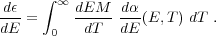
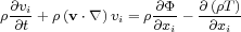
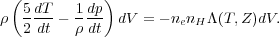
Collisional equilibrium will eventually be achieved if a plasma remains undisturbed for a long enough period of time (i.e., the inverse of the recombination rate). Several calculations have been done to determine this ionization balance as a function of the electron temperature (Jordan 1969, Arnaud & Rothenflug 1985, Arnaud & Raymond 1992, Mazzotta 1998). One such calculation is shown in Figure 2.
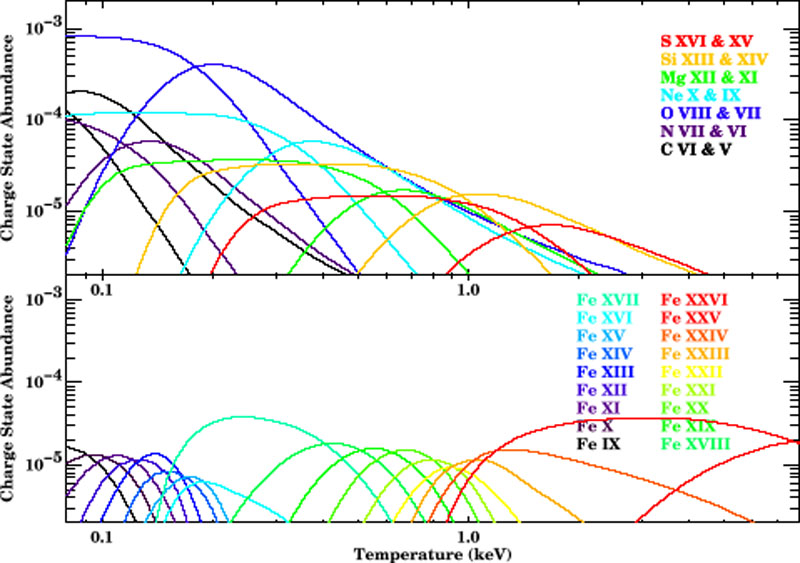 |
Figure 2. The charge state abundance (elemental abundance times fraction ionic abundance) of various ions as a function of temperature. The top panel shows helium-like and hydrogen-like charge states of various low Z atoms. The bottom panel shows iron ions having the outer electron in the K, L, and M shell. The bottom panel indicates how the measurement of various ions in the iron series is a sensitive probe of whether plasma at a given temperature exists. Figure uses data from Arnaud & Raymond (1992). |
Once the ionization balance is determined the X-ray spectrum can be calculated by considering the various radiation processes. The most important processes are bremsstrahlung and the K and L shell transitions for the discrete line emission.
3.1.3. Bremsstrahlung and other Continuum Processes
When Hydrogen is ionized above temperatures of 2 × 10⁴ K, copious amounts of bremsstrahlung emission are produced. Bremsstrahlung radiation results from the accelerations of the free electrons in the Coulomb field of an ion. The spectrum is roughly independent of energy below the energy equal to kTe, where Te is the electron temperature and k is Boltzmann's constant. A rough approximation of the power per energy per volume radiated by bremsstrahlung is given by the equation below,
 |
(4) |
where ne is the electron density, nH is the hydrogen density, E is the photon energy, k is Boltzmann's constant, and T is the electron temperature in Kelvin. The total power radiated is therefore,
 |
(5) |
In addition to bremsstrahlung, bound-free emission (the capture of a free electron to a bound state) and two-photon emission (which occurs most frequently following a collisional excitation of Hydrogen to the 2s level) are also significant source of continuum radiation. They both modify the shape of the continuum emission.
Discrete line emission is formed by a number of atomic processes. Such line emission is the most important tool for the X-ray spectroscopist. The most important atomic processes are collisional excitation, radiative recombination, dielectronic recombination, and resonant excitation. Generally, the processes have been incorporated in a number of publically available and well-tested codes that are used to study collisionally-ionized spectra.
The strength of an emission line is determined by the excitation and recombination rates, which are proportional to the integral of the velocity times the cross-section for a particular process over a Maxwellian distribution. The volume emissivity for a given emission line is calculated by equations of the form,
 |
(6) |
where CII is the rate of inner shell ionization
processes, CE is the
sum of collisional excitation processes, and
 R is the sum of
recombination processes. Several well tested codes have been developed to
calculate the emergent spectrum by assuming an ionization calculation and
including a set of excitation and recombinations rates. These include the
Raymond-Smith
(Raymond &
Smith 1977),
MEKA
(Mewe et al. 1985,
Mewe et al. 1986,
Kaastra 1992,
Mewe et al. 1995),
MEKAL
(Liedahl et
al. 1995),
and APEC codes
(Smith et
al. 2001).
These codes are compilations of the results of more detailed atomic
codes, which solve the Dirac equation either by the distorted wave
approximation
(Bar-Shalom et
al. 2001,
Gu et al. 2003]
or R-matrix methods
[Berrington et
al. 1995).
The number of transitions and the accuracy of the detailed processes
limits the results. Extensive laboratory work has been applied to verify
wavelengths
(Brown et al. 1998,
Brown et al. 2002)
and cross-sections
(Gu et al. 1999,
Chen et al. 2005)
of the transitions.
R is the sum of
recombination processes. Several well tested codes have been developed to
calculate the emergent spectrum by assuming an ionization calculation and
including a set of excitation and recombinations rates. These include the
Raymond-Smith
(Raymond &
Smith 1977),
MEKA
(Mewe et al. 1985,
Mewe et al. 1986,
Kaastra 1992,
Mewe et al. 1995),
MEKAL
(Liedahl et
al. 1995),
and APEC codes
(Smith et
al. 2001).
These codes are compilations of the results of more detailed atomic
codes, which solve the Dirac equation either by the distorted wave
approximation
(Bar-Shalom et
al. 2001,
Gu et al. 2003]
or R-matrix methods
[Berrington et
al. 1995).
The number of transitions and the accuracy of the detailed processes
limits the results. Extensive laboratory work has been applied to verify
wavelengths
(Brown et al. 1998,
Brown et al. 2002)
and cross-sections
(Gu et al. 1999,
Chen et al. 2005)
of the transitions.
A number of common spectral transitions occur in most X-ray spectra. In fact, despite the complexity implied by the above discussion there are usually only a couple of dozen strong transitions that are used to determine most of the information that can be extracted from the X-ray spectrum. Several of the important emission line blends are shown in Table 1.
| Iona | Wavelengths | Energies | Temperature | |
| Å | keV | keVb | ||
| Fe XXVI | 1.8 | 6.97 | > 3.0 | |
| Fe XXV | 1.9,1.9 | 6.70, 6.63 | 1.0
 8.0 8.0 |
|
| Fe XXIV | 10.6, 11.2 | 1.17, 1.11 | 0.9
4.0 |
|
| Fe XXIII | 11.0, 11.4, 12.2 | 1.13,1.09,1.02 | 0.8
2.0 |
|
| Fe XXII | 11.8, 12.2 | 1.05,1.02 | 0.6
1.5 |
|
| Fe XXI | 12.2, 12.8 | 1.02,0.97 | 0.5
1.0 |
|
| Fe XX | 12.8, 13.5 | 0.97,0.92 | 0.4
1.0 |
|
| Fe XIX | 13.5, 12.8 | 0.92,0.97 | 0.3
0.9 |
|
| Fe XVIII | 14.2, 16.0 | 0.87, 0.77 | 0.3
0.8 |
|
| Fe XVII | 15.0, 17.1 | 0.83,0.73 | 0.2
0.6 |
|
| 15.3, 16.8 | 0.81,0.73 | |||
| S XXVI | 4.7 | 2.62 | > 1.0 | |
| S XXV | 5.1, 5.0 | 2.43, 2.46 | 0.3
1.0 |
|
| Si XIV | 6.2 | 2.00 | > 1.0 | |
| Si XIII | 6.6, 6.7 | 1.87, 1.84 | 0.2
1.0 |
|
| Mg XII | 8.4 | 1.47 | > 0.7 | |
| Mg XI | 9.2, 9.3 | 1.35,1.33 | 0.1
0.6 |
|
| Ne X | 12.2 | 1.02 | > 0.4 | |
| Ne IX | 13.5, 13.7 | 0.92,0.90 | 0.1
0.3 |
|
| O VIII | 19.0, 16.0 | 0.64 | > 0.2 | |
| O VII | 21.6, 22.0 | 0.57, 0.56 | 0.1
0.2 |
|
| N VII | 24.8 | 0.50 | > 0.1 | |
| C VI | 33.7 | 0.37 | > 0.1 | |
| a Note this line transition list is somewhat crude since we have chosen to tabulate line blends rather than actual transitions, but matches well with the quality of the observations. | ||||
| b The temperature range is calculated to roughly show the temperature range where the emissivity of a given ion blend is within an order of magnitude of its peak emissivity. | ||||
3.1.5. X-ray Cooling Function and Emission Measure Distribution
The X-ray cooling function is calculated by integrating the emission from all processes and weighting by the energy of the photons.
 |
(7) |
where d /
dE is the energy dependent line power (or continuum
power). The cooling function relates the total amount of energy emitted per
volume for a given amount of plasma with a given temperature and emissivity.
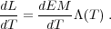
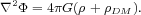
The cooling function has been compiled in various tables
(Böhringer
& Hensler 1992,
Sutherland
& Dopita 1993).
 |
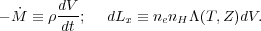
Figure 3. The radiative cooling function is shown for solar abundances (top curve), one-third solar abundances (middle), and pure Hydrogen and Helium (bottom). The X-ray region from 106 to 108 K is dominated by bremsstrahlung at high temperatures as well as significant contribution from line emission at lower temperatures. Below 106 K in the UV temperature range, the cooling function rises significantly. |
The relative distribution of plasma at a set of temperatures is often expressed in terms of an emission measure distribution. The differential emission measure, dEM / dT is defined by
 |
(8) |
where d /
dE is the energy-dependent emissivity and the integral is over
all temperatures. It is also convenient to express the distribution of
plasma temperatures in terms of the differential luminosity, which is
defined by
/
dE is the energy-dependent emissivity and the integral is over
all temperatures. It is also convenient to express the distribution of
plasma temperatures in terms of the differential luminosity, which is
defined by
 |
(9) |
The cooling time of an optically-thin plasma is the gas enthalpy divided by the energy lost per unit volume of the plasma. The gas enthalpy is 5/2 n k T and the energy lost per volume is the electron density squared times the cooling function. The cooling time can then be written as,
 |
(10) |
where tH is the age of the universe (13.7 Gyr),
T8 is the temperature in units of 108 K,
 -23 is
the cooling function in units of 10-23 ergs cm3
s-1, and
n-2 is the density in units of 10-2 particles
cm-3. We used the gas enthalpy per volume, 5/2 n
k T instead of the thermal energy per volume 3/2 n
k T
since the plasma is compressed as it cools which therefore effectively
raises its heat capacity by a factor of 5/3. Therefore,
X-ray plasma with gas density above 10-2 cm-3 has had
sufficient time to cool. In the cores of cooling clusters the cooling
time approaches cooling times below 5 × 10⁸ yr. If the
gas was undisturbed, it would have a chance to cool several times.
Note that as gas cools at constant pressure (due to the weight of
overlying gas) then the rise in density as the temperature drops means
that tcool becomes shorter and shorter.
-23 is
the cooling function in units of 10-23 ergs cm3
s-1, and
n-2 is the density in units of 10-2 particles
cm-3. We used the gas enthalpy per volume, 5/2 n
k T instead of the thermal energy per volume 3/2 n
k T
since the plasma is compressed as it cools which therefore effectively
raises its heat capacity by a factor of 5/3. Therefore,
X-ray plasma with gas density above 10-2 cm-3 has had
sufficient time to cool. In the cores of cooling clusters the cooling
time approaches cooling times below 5 × 10⁸ yr. If the
gas was undisturbed, it would have a chance to cool several times.
Note that as gas cools at constant pressure (due to the weight of
overlying gas) then the rise in density as the temperature drops means
that tcool becomes shorter and shorter.
3.1.7. Optical Depth, Resonance Scattering, and Opacity
The optical depth for photons of a given wavelength,
 , is the product of
the column density of a particular ion, Ni and the
cross-section of a particular process. The cross-section is a function
of energy. The column density is the line integral of the ion density,
ni, which is a
function of the spatial position along the line of sight.
, is the product of
the column density of a particular ion, Ni and the
cross-section of a particular process. The cross-section is a function
of energy. The column density is the line integral of the ion density,
ni, which is a
function of the spatial position along the line of sight.
The intracluster medium is, for the most part, optically-thin to its own radiation (i.e. photons escape once they are emitted without interacting again). Photons with energies close to certain resonance transitions, however, can scatter several times before leaving a cluster. The optical depth to a resonance transition is given by
 |
(11) |
where ni is the ion density,
fi is the oscillator strength of the
transition, me is the electron mass,
i is the
wavelength of the
transition, c is the speed of light, e is the electron
charge, and  i
is the line width given by,
i
is the line width given by,
 |
(12) |
where A is the atomic mass number, µ is the mean mass per particle, M is the Mach number of the turbulence or gas motions in the plasma, k is Boltzmann's constant, and T is the temperature. The above expression includes both the thermal broadening of the line as well as turbulent broadening.
If a significant quantity of lowly ionized matter exists along the line of sight, X-rays can be absorbed and re-emitted at lowly ionized longer wavelengths. This situation occurs frequently for absorption from neutral gas in the Milky Way Galaxy, but could also occur from gas trapped in the cluster potential. This subject is discussed in detail later, but we note that understanding the role of absorption often has a significant effect on the interpretation of the soft X-ray spectrum. This is particularly true at low resolution. Helium K shell absorption at low energies and Oxygen K shell absorption at 23.5 Å are the largest contributors to the opacity from a neutral absorber and produce absorption edge features in the spectrum.
The plasma of the intracluster medium can be described by magneto-hydrodynamics on large scales. Several assumptions underlie this statement. First, the ICM is optically-thin so we do not have to include radiative forces in the theory. Second, we assume the ICM is non-relativistic. This is true since the sound speed is at most a few thousand kilometers per second. Third, we assume the ICM is nearly fully-ionized, which is true since Hydrogen consitutes most of the plasma. Finally, the plasma can be treated as a fluid using continuous fields if the plasma parameter is small so that collective processes dominate. The plasma parameter is defined by
 |
(13) |
where D is
the Debye length, n is the density
in units of cm-3, and T is the temperature in K. The
ICM plasma parameter is in fact extremely small.
Magnetohydrodynamics (MHD) in this context is described by the following
variables: the fluid velocity, v, the temperature, T, the
density,
 , and the
magnetic field, B, and the dark matter density,
DM.
These quantities are related to one another
by the full set of MHD equations, which assume local thermodynamic
equilibrium of these quantities. The transport properties of the fluid
can be written in terms of the viscosity,
, and the
magnetic field, B, and the dark matter density,
DM.
These quantities are related to one another
by the full set of MHD equations, which assume local thermodynamic
equilibrium of these quantities. The transport properties of the fluid
can be written in terms of the viscosity,
 ,
conductivity, K, and resistivity,
.
,
conductivity, K, and resistivity,
.
We also adopt the following notation. T is the energy per particle;
whereas TK is the temperature in
Kelvin. They are related to one another by the
relation, T = k TK /
(µmp). k is Boltzmann's
constant, the mass of the proton is mp, and the mean
mass per particle is µmp. Additionally, the
cooling luminosity is usually defined in terms of the
electron, ne and hydrogen, nH,
number densities, which are related to the
fluid mass density by, ne = nH /
1.19 = /
(µmp).
Below are the 5 MHD equations.
 |
(14) |
 |
(15) |
 |
(16) |
 |
(17) |
 |
(18) |
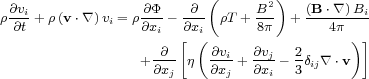
The first equation, the mass conservation equation, is a statement that the total mass of the fluid is constant. The second equation, the Navier-Stoker equation, enforces momentum conservation. This equation relates the momentum of the fluid (left hand side) to the gravitational compression (first term on the right hand side), the thermal and magnetic pressure gradients (second and third term), tangetial magnetic transport (fourth term), and viscous forces (last terms).
The evolution of the magnetic field follows the induction equation, the third equation. The first term on the right hand side generates the magnetic field due to plasma motion, and the final term dissipates the magnetic flux due to magnetic reconnection.
The energy equation, the fourth equation, expresses the balance between heating and cooling terms. The left hand side describes the energy content of the plasma (first and second term) as well as its compression (third term). The right hand side contains a conduction term (first term), a magnetic dissipation term (second term), viscous heating terms (third and fourth term), and the energy lost due to radiative cooling. In addition, this equation could include interactions between this plasma and other matter, such as dust, cosmic rays, or dark matter. Finally, the gravitational field is set by the fifth equation where both the dark matter and plasma contribute to the gravitational field.
The transport coefficients for the intracluster medium is the subject of much theoretical work. The values of these coefficients for a ionized plasma with no magnetic field was worked out by Spitzer et al. (1962) using kinetic theory. These values are given by:
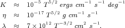 |
(19) (20) (21) |
A tangled magnetic field due to MHD turbulence, e.g. Goldreich & Sridhar (1995), could modify these coefficient considerably and there has been considerable debate in this subject (Tao 1995, Chandran & Cowley 1998, Narayan & Medvedev 2001, Maron et al. 2004). We will return to this subject in later sections.
The radiative cooling time in the cores of at least two thirds of low redshift (Peres et al. 1998) and moderate redshift (Bauer et al. 2002) clusters is less than 10 Gyr and for one third it is less than about 3 Gyr. The energy loss is directly due to the observed X-ray emission with no major bolometric correction. If there is no heating to compensate the cooling then a cooling flow occurs in these regions. In order to understand what the 'cooling-flow problem' is, why heating is required, how a 'residual flow' might operate and what happens when heating is not operating, we now briefly examine cooling flows.
The radiative cooling time tcool at tens of kpc radius in a cluster always exceeds the gravitational dynamical time so cooling leads to a slow, subsonic inflow there. The flow causes the density to rise and so maintain the pressure, which is determined by the weight of the overlying gas.
We can simplify the MHD equations significantly for the simple case of an unmagnetized single-phase subsonic flow. We also ignore any terms with conduction, viscosity, and resistivity. If we simplify the previous equations and rewrite the LHS of the energy equation based on the mass equation,
 |
(22) |
 |
(23) |
 |
(24) |
 |
(25) |
We now assume a spherical geometry and assume that the system is in a
steady-state such that the partial time derivatives can be ignored, and
assume that the flow is subsonic, then terms of order
v2 can be ignored. We combine the second equation with the
third, and define  in
the first equation, and obtain,
in
the first equation, and obtain,
 |
(26) |
 |
(27) |
 |
(28) |
 |
(29) |
When the gravitational field is important, then the temperature
approaches a critical solution which 'follows the gravitational
potential'
(Fabian et
al. 1984,
Nulsen 1986)
as can be seen from the hydrostatic equation for a power law
solution. Essentially the flow settles down to a temperature profile
close to the local virial one. In an NFW
(Navarro et
al. 1997)
potential where the inner power-law part has dark matter mass density
varying as
 r-1 this means T
r. The
temperature then flattens to T ~ 1 keV within the inner
r-1 this means T
r. The
temperature then flattens to T ~ 1 keV within the inner
 10 kpc where the gravitational potential of the central galaxy, assume
isothermal, dominates. The temperature finally collapses at the
center, before which the flow may go supersonic (the inertial velocity
term is then needed in the above momentum equation). Over most of the
region r / v
tcool, as seen in the energy equation,
which varies as T1/2 / n for
bremsstrahlung. Using the mass flow equation to substitute for v,
n
r-5/4 in the NFW case which leads to a steeper surface
brightness profile (the emissivity is proportional to
n2) than observed.
10 kpc where the gravitational potential of the central galaxy, assume
isothermal, dominates. The temperature finally collapses at the
center, before which the flow may go supersonic (the inertial velocity
term is then needed in the above momentum equation). Over most of the
region r / v
tcool, as seen in the energy equation,
which varies as T1/2 / n for
bremsstrahlung. Using the mass flow equation to substitute for v,
n
r-5/4 in the NFW case which leads to a steeper surface
brightness profile (the emissivity is proportional to
n2) than observed.
Even with the King potential commonly used before the 1990s, it was
realized that the central surface brightness was too steep to match the
observed profiles
(Fabian et
al. 1984).
Interpreted as a cooling flow, the
data indicated that the mass flow rate increased with radius (roughly
as
r out to the cooling radius rc where
tcool ~ 1010 yr). Such a situation requires
that matter is cooling out over a range of radii, which was explained by
gas with a range of densities and thus cooling times occurring at a given
radius. Therefore, more generic models than a simplified spherical
single phase flow had to be considered.
3.3.2. Thermal Instability and Multiphase flows
The above discussion of single phase flows says little about what happens on small scales. In particular, when cooling begins and what size perturbation leads to the largest growth rate and whether the multiphase flows could develop like the data seemed to indicate are an open question. There has also considerable effort to understand whether the reservoir of heat in the outer regions of clusters can be transferred to the center, which could effectively stabilize any initially thermally unstable parcels of gas.
Field (1965) originally discussed the origin of thermal instability due to the emission of radiation. He found that for all X-ray temperatures the gas is thermally unstable and the growth rate is fastest on the smallest scales. He further found that the small scale perturbations are damped by conduction so that the growth rates will be faster on somewhat larger scales. A number of authors (Malagoli et al. 1987, White & Sarazin 1987a, Balbus 1988, Loewenstein 1989, Balbus & Soker 1989) studied thermal instability in the context of gravitational field. Balbus (1991) noted that some of the thermal instability arguments are inapplicable in a cluster gravitational potential. It is possible that overdense parcels of plasma can come to equilibrium at a lower adiabat deep in the potential (Cowie et al. 1980). Kim & Narayan (2003b) argue that the radial modes are unstable even in the presence of conduction.
Nulsen (1986)
and
Thomas et
al. (1987),
however, considered the development of perturbations into cooling flows and
discussed the possible importance of magnetic fields in pinning
parcels of plasma to the general hydrodynamic flow.
Loewenstein
(1990)
discussed the importance of the magnetic field in altering the
instability conditions by effectively eliminating the buoyancy problem by
Balbus &
Soker (1989)
with magnetic stresses.
Balbus (1991)
later confirmed these
instabilities but stressed the importance of inefficient conduction
for these conditions. However a particular, and not explained,
spectrum of density perturbations is required to obtain the inferred
relation
r
(Thomas et
al. 1987,
Tribble 1989).
Binney (2004)
argues that multiphase flows do not occur in real clusters.
3.3.3. Standard Multiphase Cooling Flow Model
The standard multiphase model simplifies the physics of the flow by assuming that radiative cooling dominates the flow and then looking at the relative amount of radiation emitted at each temperature over the cooling flow volume. This can be seen as a starting point to testing the idea that cooling flows are operating in the cores of clusters. If we restore Equation 24 to the full time-derivative form and then integrate over volume and neglect any heating or additional cooling we obtain,
 |
(30) |
We define a mass loss rate per time,
, and a differential
X-ray luminosity, dLx, according to
 |
(31) |
Then the Equation 30 simplifies to,
 |
(32) |
This can be rewritten as,
 |
(33) |
In general, dp / dT will be set by the local gravitational field and magnetic pressure. If the gravitational field is relatively smooth as can be expected in dark matter haloes, then the pressure will remain nearly constant in small regions that will begin cooling. Whether this occurs depends on the development of thermal instability as discussed in the previous section. If dp / dT term is small, this expression simplifies to
 |
(34) |
which is known as the standard isobaric cooling flow model. If the density is constant which would result from high magnetic pressure, it alternatively reduces to
 |
(35) |
which is for isochoric cooling. An adiabatic equation would result if cooling were ineffective and the gravitational potential was strong and the left hand side would be zero. In general, dp / dT could be quite complicated, but note that it is fairly well established observationally that over the whole cooling flow volume the temperature derivative, dT / dr is positive and the pressure derivative is negative, dp / dr. Therefore, the last term is likely to be positive, and the relative amount of X-ray luminosity would be emitted according to somewhere in between the previous two equations if X-ray radiative cooling dominated the energy release.
Note that Equation 33 is just the first law of thermodynamics (dQ
= dU + pdV = 3/2 N k
dT +d(pV) - Vdp = 5/2 N k
dT - V d p =
5/2 N k dT - N dp /
)
differentiated with respect to
time (5/2 N k dT / dt - N /
dp /
dt kT = dQ / dt) with X-ray cooling as the
only heat loss term.
Equation 34 is also frequently expressed in terms of the emission measure,
 |
(36) |
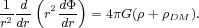
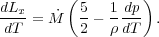
This then can be used in conjunction with the atomic physics necessary to produce an X-ray spectrum as shown in Figure 4, which can be compared with the data. X-ray spectroscopy has demonstrated that this model is incomplete and therefore we have most likely neglected additional heating or possibly cooling in our derivation of this model. The following section describes the instrumentation and analysis necessary to test it.
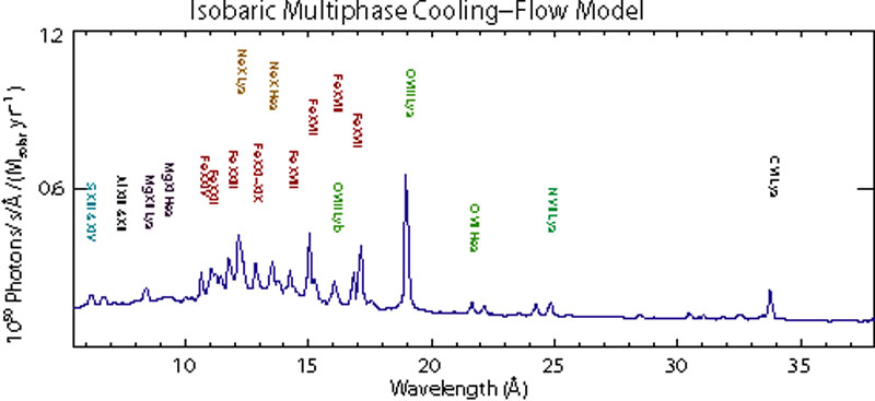 |
Figure 4. The standard isobaric cooling-flow model. The model is produced by summing collisionally-ionized X-ray spectra within a temperature range such that the relative amount of luminosity per temperature interval is a constant. This model predicts relatively prominent iron L shell transitions between 10 and 17 Å that arise from a wide range of temperatures. In particular, Fe XVII which is emitted between 500 eV and 1 keV has strong emission line blends at 15 and 17 Å. |