


It is not possible to compare the analytical work mentioned in the previous section directly with observations, because each galaxy is observed only at a single time during its evolution, and neither angular momentum exchange nor individual orbits can be directly observed. One should thus include an intermediate step in the comparisons, namely N-body simulations. In these, it is possible to follow directly not only the evolution in time, but also the angular momentum exchange and the individual orbits, i.e., it is possible to make direct comparisons of simulations with analytical work. Furthermore, one can `observe' the simulation results using the same methods as for real galaxies and make comparisons (Section 4.10). Simulations thus provide a meaningful and necessary link between analytical work and observations.
In order to show that the analytical results discussed in Section 4.5 do apply to simulations it is necessary to go through a number of intermediate steps, i.e., to show
This sequence of steps was followed in two papers (Athanassoula 2002, hereafter A02 and Athanassoula 2003, hereafter A03) whose techniques and results I will review in the next subsections, giving, whenever useful, more extended information (particularly on the techniques) than in the original paper, so that the work can be easier followed by students and non-specialists.
4.6.2. Calculating the orbital frequencies
Our first step will be to calculate the fundamental orbital
frequencies. Since we are interested in the redistribution of
Lz, we will focus on the angular and the epicyclic
frequency. The epicyclic frequency
 can be calculated with the
help of the frequency analysis technique
(Binney & Spergel 1982;
Laskar 1990),
which relies on a Fourier analysis of, e.g., the cylindrical
radius R(t) along the orbit. The desired frequency is then
obtained as the frequency of the highest peak in the Fourier
transform. The angular frequency
can be calculated with the
help of the frequency analysis technique
(Binney & Spergel 1982;
Laskar 1990),
which relies on a Fourier analysis of, e.g., the cylindrical
radius R(t) along the orbit. The desired frequency is then
obtained as the frequency of the highest peak in the Fourier
transform. The angular frequency
 is more difficult
to estimate, and in
A02
and
A03
I supplemented frequency analysis with other methods,
such as following the angle with time.
is more difficult
to estimate, and in
A02
and
A03
I supplemented frequency analysis with other methods,
such as following the angle with time.
Several technical details are important for the frequency analysis. It is
necessary to use windowing before doing the Fourier analysis, to improve the
accuracy. It is also necessary to keep in mind that some of the peaks of the
power spectrum are not independent frequencies, but simply harmonics of the
individual fundamental frequencies, or their combination. Furthermore,
if one needs considerable accuracy, one has to worry about the fact that
in standard Fast Fourier Transforms the step
d between two
adjacent frequencies is constant, while the fundamental frequencies
i will
not necessarily fall on a grid point. Except for the inaccuracy thus
introduced, this will complicate the handling of the harmonics.
between two
adjacent frequencies is constant, while the fundamental frequencies
i will
not necessarily fall on a grid point. Except for the inaccuracy thus
introduced, this will complicate the handling of the harmonics.
Frequency analysis can be applied to orbits in any analytic stationary
galactic potential, thus allowing the full calculation of the resonances
and their occupation (e.g.,
Papaphilipou & Laskar
1996,
1998;
Carpintero & Aguilar
1998;
Valluri et al. 2012).
Contrary to such potentials, however, simulations
include full time evolution, so that the galactic potential, the bar pattern
speed, as well as the basic frequencies
and
of any orbit are
time-dependent. Thus, strictly speaking, the spectral analysis technique
can not be applied, at least as such.
It is, nevertheless, possible to estimate the frequencies of a given orbit at any given time t by using the potential and bar pattern speed at this time t (which are thus considered as frozen), as I did in A02 and A03. After freezing the potential, I chose a number of particles at random from each component of the simulation and calculated their orbits in the frozen potential, using as initial conditions the positions and velocities of the particles in the simulation at time t. It is necessary to take a sufficient number of particles (of the order of 100000) in order to be able to define clearly the main spectral lines. It is also necessary to follow the orbit for a sufficiently long time (e.g., 40 orbital rotation patterns), in order to obtain narrow lines in the spectrum. By doing so I do not assume that the potential stays unevolved over such a long time. What I describe here just amounts to linking the properties of a small part of the orbit calculated in the evolving simulation potential (hereafter simulation orbit) to an equivalent part of the corresponding orbit calculated in the frozen potential. The frequencies are then calculated for the orbit in the frozen potential and attributed to the small part of the simulation orbit in question (and not to the whole of the simulation orbit). This technique makes it possible to apply the frequency analysis method, as described in A02, A03 and above, and thus to obtain the main frequencies of each orbit at a given time. It is, furthermore, possible to follow the evolution by choosing a number of snapshots during the simulation and performing the above exercise separately for each one of them. The evolution can then be witnessed from the sequence of the results, one for each chosen time.
Having calculated the fundamental frequencies as described in the
previous section, it is now possible to plot histograms of the number of
particles - or of their total mass, if particles of unequal mass are
used in the simulation - as a function of the ratio of their frequencies
measured in a frame of reference co-rotating with the bar, i.e., as a
function of ( -
p) /
. This can be carried
out separately for the particles describing the various components,
i.e., the disk, the halo, and the bulge. It was first carried out in
A02
and the results, for two different simulations, are shown in
Fig. 4.4.
 |
Figure 4.4. Number density,
NR, of particles as a function of the frequency ratio
( |
Before making this histogram, it is necessary to eliminate chaotic orbits. Their spectra differ strongly from those of regular orbits, consisting of a very large number of non-isolated lines. They of course always have a `highest peak', but this has no physical significance and is not a fundamental frequency of the orbit. Eliminating chaotic orbits is non-trivial because of the existence of sticky orbits (see Section 4.3) for which the results of the classification as regular or chaotic may well depend on the chosen integration time. Thus, although for regular orbits it is recommended to use a long integration time in order to obtain narrow, well defined spectral peaks, for sticky orbits integration times must be of the order of the characteristic timescale of the problem. For instance, if the sticky orbit shifts from regular to chaotic only after an integration time of the order of say ten Hubble times, it will be of no concern to galactic dynamic problems and this orbit can for all practical purposes be considered as regular.
It is clear from Fig. 4.4 that the
distribution of particles in
frequency is not homogeneous. In fact it has a few very strong peaks and a
number of smaller ones. The peaks are not randomly distributed; they are
located at the positions where the ratio
( -
p) /
is equal to
the ratio of two integers, i.e., when the orbit is resonant and closes
after a given number of rotations and radial oscillations. The highest
peak is at ( -
p) /
= 0.5, i.e., at the ILR. A
second important peak is located at
=
p, i.e.,
at CR where the particle co-rotates with the bar.
Other peaks, of lesser relative height, can be seen at other resonances, such as the -1/2 (OLR), the 1/4 (often referred to as the ultraharmonic resonance - UHR), the 1/3, the 2/3, etc. In all runs with a strong bar the ILR peak dominates, as expected. But the height of these peaks differs from one simulation to another and even from one time to another in the same simulation.
This richness of structures in the resonance space could have been
expected for the disk component. What, however, initially came as a
surprise was the existence of strong resonant peaks in the spheroid. Two
examples can be seen in the right-hand panels of
Fig. 4.4. In both, the strongest peak
is at corotation, and other peaks can be clearly seen at ILR, at
( -
p) /
= -0.5 (OLR) and at other
resonances. As was the case for the disk, the absolute and relative
heights of the peaks differ from one simulation to another, as well as
with time.
Thus, the results of A02 that we have discussed in this section show that, both for the disk and the spheroid component, a very large fraction of the simulation particles is at (near-)resonance. Note that this result is backed by a large number of simulations. I have analysed the orbital structure and the resonances of some 50 to 100 simulations and for a number of times per simulation. The results of these, as yet unpublished, analyses are in good qualitative agreement with what was presented and discussed in A02, A03 and here.
Further confirmation was brought by a number of subsequent and independent analyses (Martínez-Valpuesta et al. 2006; Ceverino & Klypin 2007; Dubinski et al. 2009; Wozniak & Michel-Dansac 2009; Saha et al. 2012). These studies include many different models, with very different spheroid mass profiles or distribution functions, as well as disks with different velocity dispersions. Also different simulation codes were used, including the Marseille GRAPE-3 and GRAPE-5 codes (Athanassoula et al. 1998), GyrFalcon (Dehnen 2000, 2002), FTM (Heller & Shlosman 1994, Heller 1995), ART (Kravtsov et al. 1997), Dubinski's treecode (Dubinski 1996) and GADGET (Springel et al. 2001, Springel 2005).
Note also that Ceverino & Klypin (2007) have used a somewhat different approach, and did not freeze the potential before calculating the orbits. Instead, they followed the particle orbits through a part of the simulation during which the galaxy potential (more specifically the bar potential and pattern speed) do not change too much. In this way they obtain a power spectrum with much broader peaks than in the studies that analyse the orbits in a sequence of frozen potentials. Nevertheless, the peaks are well-defined and confirm the main A02 results - namely that there are located at the main resonances - without the use of potential freezing. Note also that this version of the frequency analysis is not suitable for deciding whether a given orbit is regular or chaotic, but is considerably faster in computer time than the one relying on a sequence of frozen potentials.
4.6.4. Angular momentum exchange
In A03
I used N-body simulations to show that angular momentum is
emitted at the resonances within CR, i.e., in the bar region, and that
it is absorbed at resonances either in the spheroid, or in the disk from
the CR outwards, as predicted by analytic calculations. For this I
calculated the angular momentum of all particles in the simulation at
two chosen times t1 and t2 and
plotted their difference,
 J =
J2 - J1 as a function of the frequency
ratio ( -
p) /
of the particle orbit at
time J2. An example of the result can be seen in
Fig. 1 of
A03.
Note that particles in the disk with a positive
frequency ratio and particularly particles at ILR have
J < 0,
i.e., they emit angular momentum. On the contrary particles in the
spheroid have
J > 0,
i.e. they absorb
angular momentum and particularly at the CR, followed by the ILR and
OLR. Further asorption can be seen at the disk CR, but it is
considerably less than the amount absorbed by the spheroid. The amount
of angular momentum emitted or absorbed at a given resonance is of
course both model- and time-dependent, as were the heights of the
resonant peaks (Section 4.6.3). On
the contrary, whether a given resonance absorbs or emits is
model-independent, and in good agreement with analytic predictions
(Section 4.5).
J =
J2 - J1 as a function of the frequency
ratio ( -
p) /
of the particle orbit at
time J2. An example of the result can be seen in
Fig. 1 of
A03.
Note that particles in the disk with a positive
frequency ratio and particularly particles at ILR have
J < 0,
i.e., they emit angular momentum. On the contrary particles in the
spheroid have
J > 0,
i.e. they absorb
angular momentum and particularly at the CR, followed by the ILR and
OLR. Further asorption can be seen at the disk CR, but it is
considerably less than the amount absorbed by the spheroid. The amount
of angular momentum emitted or absorbed at a given resonance is of
course both model- and time-dependent, as were the heights of the
resonant peaks (Section 4.6.3). On
the contrary, whether a given resonance absorbs or emits is
model-independent, and in good agreement with analytic predictions
(Section 4.5).
Thinking of the bar as an ensemble of orbits, it becomes clear that there are many ways in which angular momentum can be lost from the bar region. The first possibility is that the orbits in the bar, and therefore the bar itself, will become more elongated. The second one is that orbits initially on circular orbits closely outside the bar region will loose angular momentum and become elongated and part of the bar, which will thus get longer and more massive. In both cases the bar will become stronger in the process. The third alternative is that the bar will rotate slower, i.e., its pattern speed will decrease. These three possibilities were presented and discussed in A03, where it was shown that that they are linked and occur concurrently. Thus evolution should make bars longer, and/or more elongated, and/or more massive and/or slower rotating (A03). Simulations agree fully with these predictions and go further, establishing that all these occur concurrently, but not necessarily at the same pace.
4.6.5.1. Models with maximum and models with sub-maximum disks
Since the spheroid plays such a crucial role in the angular momentum redistribution within the galaxy, it must also play a crucial role in the formation and evolution of the bar. Athanassoula & Misiriotis (2002, hereafter AM02) tested this by analysing the bar properties in two very different types of simulations, which they named MH (for Massive Halo) and MD (for Massive Disc), respectively. Both types have a halo with a core, which is big in the MD types and small in the MH ones. Thus, in MH models, the halo plays a substantial role in the dynamics within the inner four or five disk scale lengths, while not being too hot, so as not to impede the angular momentum absorption. On the contrary, in MD models the disk dominates the dynamics within that radial range.
The circular velocity curves of these two types of models are compared in Fig. 4.5. For the MD model (upper panel) the disk dominates the dynamics in the inner few disk scale lengths, while this is not the case for the MH model. MD-type models are what the observers call maximum disk models, while the MH types have sub-maximum disks. It is not yet clear whether disks in real galaxies are maximum, or sub-maximum, because different methods reach different conclusions, as reviewed, e.g., by Bosma (2002).
 |
 |
Figure 4.5. Circular velocity curves of the initial condition of two models, one of type MD (upper panel) and the other of type MH (lower panel). The solid line gives the total circular velocity, while the dashed and the dotted ones give the contributions of the disk and halo, respectively. |
As shown in AM02 and illustrated in Fig. 4.6, the observable properties of the bars which grow in these two types of models are quite different. MH-type bars are stronger (longer, thinner and/or more massive) than MD-type bars. Viewed face-on, they have a near-rectangular shape, while MD-type bars are more elliptical. Viewed side-on, they show stronger peanuts and sometimes (particularly towards the end of the simulation) even `X' shapes. On the other hand, bars in MD-type models are predominantly boxy when viewed side-on.
 |
 |
Figure 4.6. Morphology of the disk component, viewed face-on, for an MD-type (left panels) and an MH-type halo (right panels). The time in Gyr is given in the upper right corner of each panel. |
Thinking in terms of angular momentum exchange, it is easy to understand why MH-type bars are stronger than MD-type ones. Indeed, the radial density profile of MH-type haloes is such that, for reasonable values of the pattern speed, they have more material at resonance than do MD- types. Thus, all else being similar, there will be more angular momentum absorbed. This, in good agreement with analytical results, should lead to stronger bars.
It should be stressed that the above discussion does not imply that all real galaxies are either of MH type or of MD type. The two models illustrated here were chosen as two examples, enclosing a useful range of halo radial density profiles, which could actually be smaller than what is set by the two above examples. Real galaxies can well be intermediate, i.e., somewhere in between the two. It is nevertheless useful to describe the two extremes separately, since this gives a better understanding of the effects of the spheroid.
Models of MH- or MD-type which also have a classical bulge can be termed MHB and MDB, respectively. The effect of the bulge in MD models is quite strong, so that the bars in MDB models have a strength and properties which are intermediate between those of MD and those of MH types (AM02). Furthermore, A03 and Athanassoula (2007) showed that an initially non-rotating bulge absorbs a considerable amount of angular momentum - thereby spinning up - and thus a bar in a model with bulge slows down more than in a similar model but with no bulge. All this can be easily understood from the frequency analysis, which shows that there are considerably more particles at resonance in cases with strong bulges (A03; Saha et al. 2012). On the other hand, the effect of the bulge on the bars of MH types is much less pronounced.
The two models we have discussed above have a core, more or less
extended. There is a further possibility, namely that the central part
has a cusp. It has indeed been widely debated whether haloes have a cusp
or a core in their central parts. Cosmological CDM, dark matter only
simulations produce haloes with strong cusps. Thus,
Navarro et al. (1996)
find a universal halo profile, dubbed NFW profile, which
has a cusp with a central density slope
( =
dln
=
dln  / dln r) of -1.0, while
Moore et al. (1999),
with a higher resolution, find a slope of -1.5. Increasing the
resolution yet further,
Navarro et al. (2004)
found that this slope decreases with decreasing distance from the
centre, but not sufficiently to give a core. Finally, the simulations
with the highest resolution
(Navarro et al.
2010),
argue for a lower central slope
of the order of -0.7, but still too high to be compatible with a core.
/ dln r) of -1.0, while
Moore et al. (1999),
with a higher resolution, find a slope of -1.5. Increasing the
resolution yet further,
Navarro et al. (2004)
found that this slope decreases with decreasing distance from the
centre, but not sufficiently to give a core. Finally, the simulations
with the highest resolution
(Navarro et al.
2010),
argue for a lower central slope
of the order of -0.7, but still too high to be compatible with a core.
On the other hand, very extensive observational and modelling work (de Blok et al. 2001; de Blok & Bosma 2002; de Blok et al. 2003; Simon et al. 2003; Kuzio de Naray et al. 2006, 2008; de Blok et al. 2008; Oh et al. 2008; Battaglia et al. 2008; de Blok 2010; Walker & Peñarrubia 2011; Amorisco & Evans 2012; Peñarrubia et al. 2012) argues that the central parts of haloes should have a core, or a very shallow cusp, the distribution of inner slopes in the various observed samples of galaxies being strongly peaked around a value of ~ 0.2. This discrepancy between the pure dark matter, CDM simulations and observations may be resolved with more recent cosmological simulations which have high resolution and include baryons and appropriate star formation and feedback recipes. Indeed, such simulations start to produce rotation curves approaching those of observations (Governato et al. 2010, 2012; Macciò et al. 2012; Oh et al. 2011; Pontzen & Governato 2012; Stinson et al. 2012). In order to stay in agreement with observations, I will here not discuss models with cusps. Readers interested in such models can consult, e.g., Valenzuela & Klypin (2003), Holley-Bockelmann et al. (2005), Sellwood & Debattista (2006), or Dubinski et al. (2009). Let me also mention that it is possible to study models with cusps using the same functional form for the halo density as for the MH- and MD-type models (AM02), but now taking a very small core radius, preferably of an extent smaller than the softening length.
4.6.5.3. The effect of the spheroid-to-disk mass ratio
In the two models we discussed above, it is clear that it is the one with the highest spheroid mass fraction within the disk region that makes the strongest bar. Is that always the case? The following discussion, taken from A03, shows that the answer is more complex than a simple yes, or no.
Assume we have a sequence of models, all with the same total mass, i.e., that the sum of the disk and the spheroid mass within the disk region is the same. How should we distribute the mass between the spheroid and the disk in order to obtain the strongest bar? What must be maximised is the amount of angular momentum redistribution, or, equivalently, the amount of angular momentum taken from the bar region. For this it makes sense to have strong absorbers, who can absorb all the angular momentum that the bar region can emit. Past a certain limit, however, there will not be sufficient material in the bar region to emit all the angular momentum that the spheroid can absorb, and it will be useless to increase the spheroid mass further. So the strongest bar will not be obtained by the most massive spheroid, but rather at a somewhat lower mass value, such that the equilibrium between emitters and absorbers is optimum and the angular momentum exchanged is maximum. For the models discussed in AM02 and A03, this occurs at a spheroid mass value such that the disk, in the initial conditions, is sub-maximum. In Section 4.9.3 we will discuss how disks may evolve from sub-maximum to maximum during the simulation.
In the previous sections I reviewed the very strong evidence accumulated so far showing that many particles in the simulations, both in the disk and the spheroid component, are on (near-)resonant orbits and that the angular momentum exchanged between them is as predicted by the analytic calculations, i.e., from the bar region outwards (Section 4.5). The next step should be to clarify the importance of the halo resonances in the evolution. For this we have to compare two simulations, one in which the halo resonances are at work and another where they are not, as was first done in A02, whose main results will be reviewed here.
Each of the Fig. 4.7 and 4.8 compares two models with initially identical disks. In other words, the particles in the disk initially have identical positions and velocities in the two compared simulations. The models of the haloes were also identical, but in one of the simulations (right-hand panels) the halo was rigid (represented only by the forces that it exerts on the disk particles) and thus did not evolve. In the other one, however, the halo was represented by particles, i.e., was live (left-hand panels). These particles move around as imposed by the forces and can emit or absorb angular momentum, as required.
Figure 4.7 compares the disk evolution in the live and in the rigid halo when the model is of MH type. The difference between the results of the two simulations is stunning. In the case with a live halo a strong bar has formed, while in the case with a rigid halo there is just a very small inner oval-like perturbation. This shows that the contribution of the halo in the angular momentum exchange can play an important role, actually, in the example shown here, the preponderant role.
 |
Figure 4.7. Comparison of the evolution of the bar in a live halo (left-hand panel) to that in a rigid halo (right-hand panel) for an MH-type halo. |
Figure 4.8, shows the results of a similar experiment, but now in an MD-type halo. The difference is not as stunning as in the previous example, but is still quite important. In the live halo case the bar is considerably longer and somewhat thinner than in the case with a rigid halo.
 |
Figure 4.8. Comparison of the evolution of the bar in a live halo (left-hand panel) to that in a rigid halo (right-hand panel) for an MD-type halo. |
It is thus possible to conclude that the role of the halo in the angular momentum redistribution is important. In fact in the MH-type models the role of the halo is preponderant, but it is still quite important even in the MD-types. It is thus strongly advised to work with live, rather than with rigid haloes in simulations.
4.6.7. Distribution of frequencies for MD- and MH-type models
Figure 4.4 displays the frequency histograms for two models, one MD-type (upper panels) and one MH-type (lower panels). The properties of these two types of models were discussed in Section 4.6.5.1, where their initial rotation curve, as well as their bar morphology are also displayed.
It is now useful to compare the distribution of frequencies for the two simulations used in Fig. 4.4. Starting with the disk we note that the ILR peak is about 50% higher in the MH than in the MD model, while the CR peak is considerably lower. Also the MD model has an OLR peak, albeit small, while none can be seen in the MH one. For the spheroid, the strongest peak for both models is the CR one, which is much stronger in the halo than in the disk. It is, furthermore, stronger in the MH than in the MD model. Also the MH spheroid has a relatively strong ILR peak, which is absent from the MD one. On the other hand, the MD model has a much stronger OLR peak than the MH one.
All these properties can be easily understood. From Fig. 4.6 it is clear that the bar in the MH model is stronger than in the MD one, as discussed already in Section 4.6.5.1, and this accounts for the much stronger ILR peak for the disk of the MH model. Also, from the initial circular velocity curves (Fig. 4.5) it is clear that the halo of the MH model has much more mass than the MD model within the radial extent where one would expect the CR and particularly the ILR to be. This explains why the CR halo peaks are stronger in the MH model and why the halo ILR peak is absent in the MD one. At larger radii the order between the masses of the MH and the MD haloes is reversed, being in the outer parts relatively larger in the MD model. This explains why the halo OLR peak is stronger for the MD halo than for the MH one.
4.6.8.1. Evolution of the bar strength with time
Figure 4.9 shows the evolution of the bar strength 6 with time, comparing an MH-type and an MD-type model. It clearly illustrates how important the differences between these two types can be, as expected. It also shows that, in both cases, one can distinguish several evolutionary phases.
 |
Figure 4.9. Evolution of the bar strength with time for two models, one of the MD-type (dashed line) and the other of the MH type (solid line). |
By construction, both simulations start axisymmetric and this lasts all through what we can call the pre-growth phase. The duration of this phase, however, is about half a Gyr for the MD model, while for the MH one it lasts about 2 Gyr. The second phase is that of bar growth, and lasts considerably less than a Gyr for the MD model and much longer (about 2 Gyr) for the MH one. In total, we can say that the bar takes less that 1 Gyr to reach the end of its growth phase in the MD model, compared to about 4 Gyr in the MH one. This is in good qualitative agreement with what was already found by Athanassoula & Sellwood (1986), using simpler 2D simulations. From this and many other such comparisons, it becomes clear that the presence of a massive spheroid can very considerably both delay and slow down the initial bar formation due to its strong contribution to the total gravitational force.
After the end of the bar growth time, both models undergo a steep drop of the bar strength. This is due to the buckling instability (Raha et al. 1991). The final phase - which can also be called the secular evolution phase - starts somewhat after 5 Gyr for the MH model and after about 3 Gyr for the MD one. The corresponding bar strength increase which takes place during this phase is much more important for the MH than for the MD mode. By the end of the evolution, MH models have a much stronger bar than MD ones. As already mentioned, this is due to the more important angular momentum redistribution in the former type of models.
As in Section 4.6.5.1, let me stress that we are comparing two models which display strong differences. Real galaxies can be of either type, but, most probably, can be intermediate, in which case their bar strength evolution would also be intermediate between the two shown in Fig. 4.9.
4.6.8.2. Spheroid mass and bar strength
Figure 4.9 illustrates another important point, first argued in A02, namely that the effect of the spheroid on the bar strength is very different, in fact opposite, in the early and late evolutionary stages.
4.6.8.3. Velocity dispersion and bar strength
Analytical works for the disk and/or the spheroidal component (Lynden-Bell & Kalnajs 1972; Tremaine & Weinberg 1984; A03) predict that the hotter the (near-)resonant material is, the less angular momentum it can emit or absorb. This was verified with the help of N-body simulations in A03. Contrary to the spheroid mass, velocity dispersion has the same effect on the bar strength evolution both in the early bar formation stages and in the later secular evolution stages. In the early stages a high velocity dispersion in the disk slows down bar formation, as shown initially by Athanassoula & Sellwood (1986) and later in A03. This is illustrated also in Fig. 4.10, where I compute two MD-type models with different velocity dispersions. The first one has a Toomre Q parameter (Toomre 1964) of 1.3 and the second one of 1.7. This difference has a considerable impact on the growth and evolution of the bar. In the former the bar starts growing after roughly half a Gyr, its growth phase lasts about 1.5 Gyr and the secular increase of the bar strength starts around 4.5 Gyr. For the latter (hotter) model the beginning and end of each phase are much less clear, so that one can only very roughly say that the bar growth starts at about 4, or 5 Gyr and ends at about 9 Gyr. During the later evolutionary stages also, a high velocity dispersion will work against an increasing bar strength because, as shown by analytic work and verified by N-body simulations, material at resonance will emit or absorb per unit mass less angular momentum when it is hot.
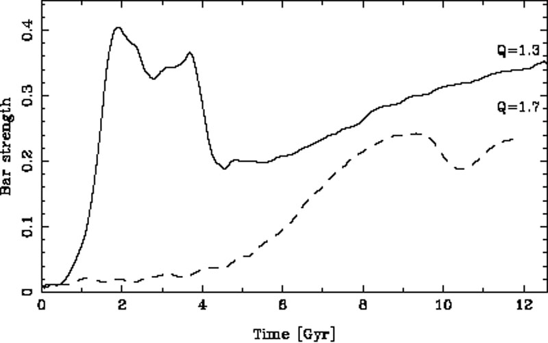 |
Figure 4.10. Evolution of the bar strength with time for two models with different Toomre Q parameters. Both models are of MD type. |
Thus, increasing the velocity dispersion in the disk and/or the spheroid leads to a delayed and slower bar growth and to weaker bars. This has important repercussions on the fraction of disk galaxies that are barred as a function of redshift and on their location on the Tully Fisher relation (Sheth et al. 2008, 2012).
4.6.8.4. Bar strength and redistribution of angular momentum
One of the predictions of the analytic work is that there is a strong link between the angular momentum which is redistributed within the galaxy and the bar strength. One may thus expect a correlation between the two if the distribution functions of the disks and spheroids of the various models are not too dissimilar. This was tested out in A03, using a total of 125 simulations, and was found to be true. Here we repeat this test, using a somewhat larger number of simulations (about 400 instead of 125) and a more diverse set of models and again a good correlation is found. The result is shown in Fig. 4.11, where each symbol represents a separate simulation. It is clear that this correlation is tight, but still has some spread, due to the diversity of the models used. Note also that we have not actually used the total amount of angular momentum emitted from the bar region (or, equivalently, the amount of angular momentum absorbed in the outer disk and in the spheroid), but rather the fraction of the total initial angular momentum that was deposited in the spheroid, which proves to be a good proxy to the required quantity. Finally, note that the points are not homogeneously distributed along the trend. This has no physical significance, but is simply due to the way that I chose my simulations. Indeed I tried to study the MH-type and the MD-type models and was relatively less interested in the intermediate cases.
 |
Figure 4.11. Bar strength,
SB, as a function of the amount of angular
momentum absorbed by the spheroid,
|
6 The definition of bar strength is not unique. The one used in the analysis of simulations is usually based on the m = 2 Fourier component, but precisely how this is used varies from one study to another. We will refrain from giving a list of precise definitions here, as this would be long and tedious. Furthermore we will, anyway, only need qualitative information for our discussions here, which is the same, or very similar, for all definitions used in simulations. We will thus talk only loosely about `bar strength' here and use arbitrary units in the plots (see also Section 4.10). Back.