Annu. Rev. Astron. Astrophys. 2009. 47: 159-210 Copyright © 2009 by Annual Reviews. All rights reserved

2. A GLOBAL VIEW OF GALAXY PROPERTIES

A breakthrough of recent surveys has been the ability to explore many dimensions of galaxy properties simultaneously and homogeneously, in order to put galaxy scaling relationships in context with respect to one another. In this section, we describe these general properties, their distribution, and their dependence on environment. We concentrate in this section primarily but not exclusively on SDSS results, which currently yield the most homogeneous and consistent measurements for the broadest range of galaxy varieties. In particular, in the subsections below we will make use of 77,153 galaxies with z < 0.05 in the SDSS Data Release 6 (DR6; Adelman-McCarthy et al. 2008), an update of the low-redshift sample of Blanton et al. (2005c).

2.1. Optical broad-band measurements

Figure 1 shows the simplest measurable properties of galaxies from the SDSS sample: the absolute magnitude M_r, the g-r color, the Sérsic (1968) index n in the r-band, and the physical half-light radius r₅₀ (sometimes called the "effective radius"). These properties reveal a variety of correlations, most known for many years, but now quantified much more precisely.

Figure 1. Distribution of broad-band galaxy properties in the SDSS. The diagonal panels show the distribution of four properties independently: absolute magnitude Mr, g-r color, Sérsic index n, and half-light radius r50. A bimodal distribution in g-r is apparent. The off-diagonal panels show the bivariate distribution of each pair of properties, revealing the complex relationships among them. The greyscale and contours reflect the number of galaxies in each bin (darker means larger number).

The absolute magnitude M_r is a critical quantity, correlating well with stellar mass as well as with dynamical mass (see the discussion of the Tully-Fisher relation in Section 3.9 and the fundamental plane in Section 5.4). Clearly, the other properties are a strong function of overall mass. Although Figure 1 shows the raw distribution for the flux-limited SDSS sample, in Section 2.3 we correct for selection effects and calculate the luminosity and stellar mass functions.

In many of these plots, particularly those involving g-r color, there is a bimodal distribution - galaxies can be divided very roughly into red and blue sequences (Strateva et al. 2001, Blanton et al. 2003, Baldry et al. 2004). The red and blue classification is not always related in a simple way to classical morphology - though of course there is some relationship (Roberts & Haynes 1994). In particular, galaxies in the blue sequence are very reliably classifiable as spiral galaxies with ongoing star-formation (Section 3). However, the red sequence contains a mix of types. The lower luminosity end consists of compact ellipticals (cEs) and dwarf ellipticals (dEs; sometimes known as spheroidals, Sph). Around M_r - 5log₁₀ h ~ -20, the red sequence is a mix of early-type spirals, dust-reddened spirals (Section 3.6), lenticulars (S0s; Section 4), and giant ellipticals (Es; Section 5). At the highest luminosities, it consists of cD galaxies (Section 5.5).

For a rough quantification of how these types populate the red sequence, we use the classifications of our sample galaxies stored in the NASA Extragalactic Database (NED). In practice, most of these classifications come from The Third Reference Catalog of Bright Galaxies (RC3; de Vaucouleurs et al. 1991). For our purposes we select galaxies within (g-r) ~ 0.03 of the red sequence, with no detected lines associated with star-formation (see Section 2.2 and Figure 2). For any luminosity M_r - 5log₁₀h < -17, only about 40% of these galaxies are Es. About 25%-50% of them are S0s, with the lowest fractions at around M_r - 5log₁₀ h ~ -20, increasing to both higher and lower luminosities. We suspect these fractions are in practice overestimates, since spiral systems are far more commonly misclassified as E/S0s than vice-versa. It remains clear, however, that restricting to red sequence galaxies does not suffice to guarantee an E/S0 sample - at M_r - 5log₁₀ h ~ -20 at least one-third of the red sequence population is Sa or later.

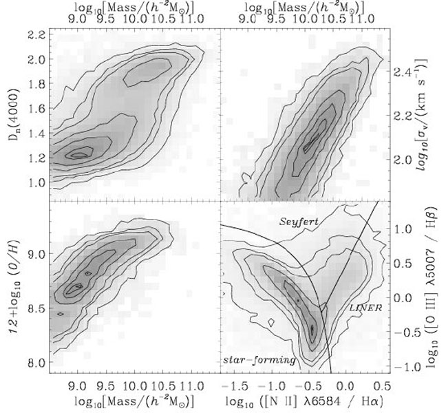Figure 2. Distribution of spectroscopic galaxy properties in the SDSS (data courtesy Brinchmann et al. 2004, Tremonti et al. 2004). Greyscale and contours are similar to those in Figure 1. Upper left panel shows the distribution of stellar mass and Dn(4000), a measure of the stellar population age. As in the color-magnitude diagram, the separation between old and young populations is apparent. Upper right panel shows for red galaxies the distribution of stellar mass and velocity dispersion, revealing the Faber-Jackson relation. Bottom left panel shows for star-forming galaxies the relationship between mass and gas-phase oxygen abundance, the "mass-metallicity" relation. Bottom right panel shows the Baldwin, Phillips & Terlevich (1981) relationship for emission-line galaxies. Shown are the divisions (based on Kauffmann et al. 2003a) among star-forming, Seyfert, and LINER galaxies.

Both the red and blue sequences have mean colors that are a function of absolute magnitude. Blue galaxies have recent star-formation, and their color is strongly related to the recent star-formation history (Section 3.5) and the dust reddening in the galaxy (Section 3.6). As galaxy mass increases, the change in color reflects both the increased reddening due to dust and the decreased fraction of recent star-formation (related to an increased importance of red central bulges; Section 3.3). The strong dependence on recent star formation history translates into the large range of colors on the blue sequence. As one might expect given this trend, at high masses the atomic and molecular gas fractions are low (Section 3.4), whereas the metallicities are high (Section 3.7).

Red galaxies have (generally) little recent star-formation, and their color is weakly related to both mean stellar age and to metallicity, both of which rise with mass (Section 5.7). Because the dependence of color on these properties is weak relative to their intrinsic variation, there is a small range of red galaxy colors in Figure 1. Although their old stellar age is related to their relatively gas-poor nature, they are not entirely devoid of cold gas (Section 5.8) or perhaps of relatively recent star-formation (Section 5.7).

The Sérsic index n is a measurement of the overall profile "shape," and is defined by the profile:

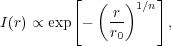(1)

where r₀ is a scale factor that one can relate to the half-light radius r₅₀ given n (Sérsic 1968; see Graham & Driver 2005 for the mathematical relationship). In general, this model is usually generalized to non-axisymmetric cases by allowing for an axis-ratio b / a < 1 (that is, elliptical rather than circular isophotes). While r₅₀ reflects the physical size of the galaxy, n reflects what we define as the "concentration." As n→ 0, the Sérsic profile approaches a uniform disk of light with radius r₀. As n increases, the Sérsic function simultaneously concentrates the surface brightness profile towards the center and pushes flux further out, passing through a Gaussian (n = 0.5), an exponential (n = 1), a de Vaucouleurs profile (n = 4; de Vaucouleurs 1948), and even higher for some galaxies. This index often is used as a proxy for morphology (e.g., Bell et al. 2003, Shen et al. 2003, Mandelbaum et al. 2006), though it is only partially related to classical morphological determinations (Section 3.2).

For many galaxies a single Sérsic index model does not explain the profile completely. For elliptical galaxies, the central regions are often not well fit by such a model (Section 5.3). For spiral and lenticular galaxies a better model is an exponential disk plus a Sérsic bulge (Section 3.3). However, as Graham (2001) shows, measures of the overall concentration are well-correlated with bulge-to-disk ratios for real galaxies.

Consequently, in Figure 1 the single component Sérsic n does reveal some interesting trends. Blue galaxies generally have low Sérsic indices, while red galaxies span a range of Sérsic indices. Overall, both blue galaxies and red galaxies tend to be more concentrated at higher luminosity. For blue galaxies this reflects an increased importance of the bulge, and a simultaneous increase in concentration of the bulge itself (Section 3.3). For red galaxies the trend appears to reflect an overall structural difference between low luminosity and high luminosity early-type galaxies (Section 5.2).

Finally, the plots also demonstrate that the optically emitting regions of galaxies are larger for more massive galaxies. Luminous galaxies achieve r₅₀ > 10 h^-1 kpc, while the low luminosity population typically has r₅₀ < 1 h^-1 kpc. The full extent of the galaxies in the optical tends to be at least 2-4 × r₅₀ for most systems depending on the concentration. For disk galaxies, even this optical radius does not trace the outer gas disk often visible in Hi and in very sensitive ultraviolet (UV) measurements (Section 3.8).

2.2. Optical spectroscopic measurements

More detailed information on stellar populations and the interstellar medium can be obtained from integrated spectrophotometry (Kennicutt 1992, Jansen et al. 2000, Moustakas, Kennicutt & Tremonti 2006). In Figure 2, we show a small sampling of the major trends in galaxy spectroscopic properties in the optical, using the same sample as in Figure 1, with parameters determined by Brinchmann et al. (2004) and Tremonti et al. (2004) for our SDSS sample. The SDSS spectra are taken through 3 arcsec diameter fibers, a generally small radius within nearby galaxies, and so aperture effects are not ignorable; however, the general conclusions we draw here are not affected much by this consideration.

For the purposes of these plots, we replace luminosity by the stellar mass. There are numerous methods for calculating stellar mass; see the compilation of major techniques in Baldry, Glazebrook & Driver (2008). Here we use the simple technique of Bell et al. (2003), which assigns a mass-to-light ratio according to the galaxy broad-band colors. This technique is robust at least for most galaxies, because in practice increasing dust, age, and metallicity all both increase the mass-to-light ratio and redden the colors, in roughly similar proportions. Of course, galaxies with large, recent bursts of star-formation or extreme amounts of dust attenuation will not be well-described by this simple technique (Bell & de Jong (2001)). But the greater unknown in determining stellar masses is the initial mass function (IMF) of stars assumed, because the lowest mass stars contribute considerable mass but very little light. In fact, as Baldry, Glazebrook & Driver (2008) show, a number of disparate techniques for calculating stellar masses agree well at fixed IMF. The Bell et al. (2003) estimate we use employs the non-physical "diet" Salpeter IMF, which yields stellar masses slightly higher (~ 0.05 dex) than the popular Kroupa (2001) and Chabrier (2003) IMFs.

The upper left panel of Figure 2 shows the distribution of stellar mass and the quantity D_n(4000), a measure of the 4000-Å break, according to the "narrow" definition of Balogh et al. (1999) and using the determination of Brinchmann et al. (2004). As Kauffmann et al. (2003b) point out, the 4000-Å break traces stellar population age better than broad-band colors, and it is less sensitive to dust reddening. Star-forming galaxies tend to have weak breaks, with D_n(4000) ~ 1.1-1.4, whereas passive stellar populations tend to have strong breaks, with D_n(4000) ~ 1.8-2.1. Indeed, similar to galaxy color, D_n(4000) clearly separates these two populations; older populations dominate at high stellar mass and the star-forming systems dominate at low stellar mass. Based on this diagram, Kauffmann et al. (2003) define a critical stellar mass of 1.5 × 10¹⁰ h^-2 M separating these two galaxy populations.

From SDSS spectra, we can also determine galaxy velocity dispersions; for a sample of galaxies without emission lines, we show the results in the upper right panel of Figure 2. Here we see a clear correlation between velocity dispersion and stellar mass, related of course to the classic relation of Faber & Jackson (1976). This relationship is merely a projection of the fundamental plane (Section 5.4). Both the fundamental plane and the Tully-Fisher relation (Section 3.9) show that the dynamical masses of galaxies are correlated with their stellar masses.

The bottom right panel of Figure 2 shows the "BPT" diagram (Baldwin, Phillips & Terlevich 1981), based on the H and H recombination lines and the [N ii] 6584 and [O iii] 5007 collisionally excited forbidden lines. The position of an object in the BPT diagram is a function of metallicity and the ionization state of the emitting gas (e.g, Kennicutt et al. 2000) and can be roughly divided into three regions (following Kauffmann et al. 2003a). The lower left region contains emission line galaxies dominated by star-formation. The upper triangle contains Seyfert galaxies, which have higher ionizing fluxes and are likely associated with AGN. The lower right contains Low Ionization Nuclear Emission-line Regions (LINERs; Heckman 1980, Kewley et al. 2006), also most likely associated with AGN. Ho (2008) discuss the classification and physical properties of nearby AGN in much greater detail than possible here.

Finally, we isolate the star-forming galaxies (those with emission lines falling in the star-formation region of the BPT diagram). The lower left panel of Figure 2 shows their gas-phase metallicity (from Tremonti et al. 2004). We use the standard quantification of oxygen abundance, 12 + log₁₀(O/H). Clearly more massive galaxies are more metal-rich, saturating around 9.2 dex (about 0.5 dex more oxygen-rich than the newly revised solar abundance; Meléndez & Asplund 2008). Closed-box chemical evolution models do predict an increase in metallicity as the fraction of gas turned into stars rises, since more generations of star-formation have occurred. However, in fact, the observed increase in metallicity is likely also driven by metal-rich outflows in low-mass galaxies, or another violation of the closed-box model (Section 3.7).

2.3. Luminosity and stellar mass functions

A fundamental measurement of the galaxy distribution is the luminosity function (LF): the number density as a function of luminosity. With flux-limited samples, such as those shown in Figures 1 and 2, one needs to apply corrections for the fact that faint galaxies cannot be observed throughout the survey volume. A number of statistical techniques have been developed over the years to correct for this effect, the simplest of which is the 1 / V_max method (Schmidt 1968). Using this method, one counts each galaxy with a weight equal to the inverse of the volume over which it could have been observed. In the integral over volume, one must include any weighting for survey completeness as well as flux or other selection effects, based on the galaxy's particular properties. Then, in any bin of any set of properties one can calculate the number density of galaxies in that bin as _i 1/V_max,i. For modern samples, the results from this method agree with others designed to be insensitive to accidental correlations between large-scale structure and redshift (e.g. Efstathiou, Ellis & Peterson 1988, Takeuchi, Yoshikawa & Ishii 2000).

The upper left panel of Figure 3 shows the optical r-band LF from the SDSS DR6 sample, using V_max calculations described in Blanton et al. (2005b). We show both the overall LF and the LF split among galaxy types, using some very basic criteria. The "late" population consists of any blue galaxies plus any star-forming red galaxies. The "early" population consists of other galaxies, split into concentrated early-types, which have n > 2, and diffuse early-types, with n < 2. These classifications are crude, of course - this method describes many legitimate Sa galaxies and basically all S0 galaxies as "early-type," for example.

Figure 3. Optical and near-UV luminosity function, stellar mass function, and H i mass function of galaxies. The upper left panel shows the local r-band luminosity function of all galaxies (black histogram), as well as the luminosity functions of late-types (blue), concentrated early-types (red) and diffuse early-types (orange), as described in Section 2.3. Overplotted as the smooth curve is the double Schechter function fit of Blanton et al. (2005b). The upper right panel shows the local stellar mass function for the same galaxies. The bottom left panel shows the GALEX near-UV luminosity function for the various galaxy types and the smooth fit to the full luminosity function from Schiminovich et al. (2007). Finally, the lower right panel shows the H i mass function fits from Springob, Haynes & Giovanelli (2005) for all galaxies and as a function of morphological type.

Nevertheless, this panel begs comparison with Figure 1 of Binggeli, Sandage & Tammann (1988), who show very similar trends in the LF using visual morphological classifications. As they found, early type galaxies dominate the bright-end, while late-types dominate the faint end. Diffuse early-types become increasingly important at low luminosity.

As Binggeli, Sandage & Tammann (1988) also showed, a Schechter (1976) function fit to the LF is insufficient. We overplot the double-Schechter function fit of Blanton et al. (2005b), which uses a broken power-law for the faint end:

(2)

The parameter L_∗ is a fundamental one, indicating the approximate onset of the exponential cut-off. At the faint-end the luminosity function is approximately a power law with slope ₂ ranging between -1.35 and -1.52 in the r-band depending upon assumptions about the low surface brightness population (Section 2.4).

The upper right panel of Figure 3 shows the stellar mass function, using the same stellar mass determinations as used in Figure 2. Because the stellar mass-to-light ratios of red galaxies are higher than blue galaxies, the stellar mass function accentuates the distinction between the blue and red populations: the early-types become even more dominant. Overlaid is the double Schechter fit of Baldry, Glazebrook & Driver (2008), who present a comprehensive treatment of recent estimates of the stellar mass function (the results shown here use the Chabrier (2003) IMF). After accounting for differences in the adopted IMF, these results are in rough agreement with determinations of Cole et al. (2001), Kochanek et al. (2001), and Bell et al. (2003) based on 2MASS K-band data.

The lower left panel of Figure 3 shows the near-UV luminosity function, which traces recent star-formation, obtained by matching the SDSS sample to the GALEX Release 3 (GR3; Martin et al. 2005). We separate the galaxies according to the same classifications as used above. We K-correct here to the near-UV band shifted blueward by a factor 1 + z = 1.1 (Blanton & Roweis 2007) for consistency with Schiminovich et al. (2007). Overlaid as the smooth black line is their full luminosity function. Clearly the early-types are very subdominant - the UV luminosity of the Universe is completely dominated by blue, star-forming galaxies.

Finally, in the lower right panel of Figure 3 we show the Hi mass functions determined by the compilation of Springob, Haynes & Giovanelli (2005), which is comparable to the HIPASS result of Zwaan et al. (2005). Since they did not publish their full functions, we only show the Schechter function fits (which are accurate descriptions). They limited their sample to spiral galaxies; most ellipticals have very low atomic gas content and would not contribute significantly to this plot (Section 5.8), though they often have significant hot ionized gas (Mathews & Brighenti 2003). They split the sample according to morphological type (though virtually all of the types would fall into the "late-type" histograms in the other plots). The most notable effect is that the mass cut-off scale for the Hi mass function is far lower than for the stellar mass function: the most massive galaxies are dominated by stars, not neutral hydrogen. That situation changes dramatically at lower masses (Section 3.4).

2.4. Systematic effects in luminosity functions

For the luminosity and stellar masses in this section, we relied upon SDSS Petrosian magnitudes (Petrosian 1976, Blanton et al. 2001, Strauss et al. 2002), which have the virtue that they are roughly redshift-independent quantities. Some researchers advocate the use of "total" flux, using extrapolated radial profiles. The difference is largest for de Vaucouleurs profiles (with SDSS Petrosian fluxes less by 10%-20%, depending on the ratio of the half-light radius to the seeing). For very detailed work, such as the build-up of stellar mass on the red sequence, it is therefore necessary to know the flux estimator used (e.g., Brown et al. 2007). In the context of SDSS, another problem exists: the biggest galaxies on the sky have their fluxes significantly underestimated owing to oversubtraction of the background (Blanton et al. 2005a, Bernardi et al. 2007), yielding a 20% bias at r₅₀ ~ 20'' and rising at larger sizes (Lauer et al. 2007b). For that reason, the effect on the luminosity function is minimal, since virtually all of the brightest galaxies in the sample are far away and thus small in angular size.

All luminosity and stellar mass function estimates are affected at some level by surface brightness selection effects. Blanton et al. (2005c) estimate that for the SDSS these effects become important at the 10% level at M_r - 5log₁₀ h ~ -17 or so. At lower luminosities, the SDSS spectroscopic survey starts to become incomplete; for 2MASS-based surveys like Cole et al. (2001) or Kochanek et al. (2001), the incompleteness probably sets in at higher luminosities, though no quantitative estimate exists. A less traditional view is that of O'Neil et al. (2004), who suggest that a substantial reservoir of baryons could be in massive low surface brightness galaxies, with large H i masses (> 10¹⁰ M) but barely detectable in optical surveys. Such galaxies exist, but no quantitative estimate of their number density has been made.

2.5. Environmental dependence

As has long been established, all of these properties are a strong function of the local environment - whether a galaxy is in a cluster or in a void. With the latest data sets, we now have a much more detailed understanding of this dependence. To illustrate these effects, we estimate environment using the number N_n of neighboring galaxies with M_r - 5log₁₀ h < -18.5, within a projected distance of 500 h^-1 kpc and a velocity of 600 km s^-1. The luminosity threshold is roughly that of the Large Magellanic Cloud. Other measures of galaxy environment have been explored recently: group environment (Yang et al. 2007), nearest neighbor distance (Park et al. 2007), and kernel density smoothing (Balogh et al. 2004). The results we describe here seem to hold no matter which estimate of density one uses.

First, let us consider the variation of the stellar mass function with environment, as shown in Figure 4. The panels are broken up, as labeled, into bins of N_n - the upper right panel is roughly the environment of galaxies in the Local Group. The first notable fact is that most galaxies with 0.01 L_∗ L L_∗ are in relatively underdense environments, at the scale of the Local Group or less. Generally speaking, the massive galaxies are relatively more likely to exist in dense regions, reflecting the variation of the shape of the optical luminosity function from void regions (Hoyle et al. 2005), through average regions (Blanton et al. 2005c), to clusters (Popesso et al. 2005).

Figure 4. Stellar mass function of galaxies as a function of morphological type (see Fig. 3 and Section 2.3) and local galaxy density. Each panel corresponds to a different environment, ranging from isolated, to poor groups, rich groups, and clusters, based on the number of neighbors Nn with Mr - 5log10 h < -18.5 within 500 h-1 kpc and 600 km s-1. For reference, this luminosity threshold roughly corresopnds to the luminosity of the Large Magellanic Cloud. The double Schechter function fit to all galaxies from Baldry, Glazebrook & Driver (2008) is shown in all panels as a smooth black curve.

Second, let us consider the more detailed properties of galaxies as a function of environment. For example, Figure 5 shows the relationship between D_n(4000) and stellar mass as a function of environment. For reference, we show the rough location of each galaxy sequence as the red and blue lines, identically in each panel of Figure 5. Though the position of each sequence changes only a little with environment, how each sequence is populated changes considerably, with old galaxies preferentially located in dense regions, as found for these parameters by Kauffmann et al. (2004).

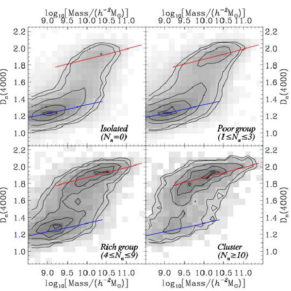Figure 5. Distribution of Dn(4000) and stellar mass as a function of environment as defined in Section 21. In each panel we show references for the young and old galaxy sequences as the blue and red lines, respectively.

Other measurements of the change of galaxy properties with environment track this same segregation of galaxy types: broad-band color and Sérsic index (e.g., Hashimoto & Oemler 1999, Blanton et al. 2005a, Yang et al. 32007); H emission, star-formation rate, and other spectral properties (e.g., Lewis et al. 2002, Norberg et al. 2002, Gomez et al. 2003, Boselli & Gavazzi 2006); and of course classical morphology (e.g., Dressler 1980, Postman & Geller 1984, Guzzo et al. 1997, Giuricin et al. 2001). It appears that among all these properties, the controlling variables are those related to mass and star-formation history - not those having to do with structure (Kauffmann et al. 2004, Blanton et al. 2005a, Christlein & Zabludoff 2005, Quintero et al. 2006).

Figure 6 demonstrates this conclusion. The top two rows compare the relationship between Sérsic index and stellar mass for a "young" population and an "old" population, where the division is taken to be at D_n(4000) = 1.6. Each relationship remains remarkably fixed as a function of density. This means that once the stellar population age and stellar mass are fixed, the environment of a galaxy does not relate to its overall structure. In contrast, if we classify galaxies according to Sérsic index, their stellar population ages are a strong function of environment.

Figure 6. Demonstration of the asymmetric relations between structure and star-formation history. Each column isolates a range of densities using the number of neighbors Nn, as defined in Section 2.5. The top two rows show the relationship between Sérsic index and stellar mass in an "old" sample and a "young" sample. For the old sample plots, the red line remains the same in all plots. For the young sample plots, the blue line remains the same. The bottom two rows show the relationship between Dn(4000) and stellar mass in a "concentrated" sample and a "diffuse" sample. At fixed Sérsic index the stellar population ages clearly depend strongly on density (even at fixed mass). However, at fixed stellar population age, the Sérsic index does not vary significantly with density.

This theme persists for almost all properties of galaxies as a function of environment. Once galaxies are appropriately classified - that is, by some parameter related to the star-formation history - then galaxy scaling laws are usually weak functions of environment. For example, Park et al. (2007) classified galaxies by color and color gradient, and explored the scaling relationships of each type thoroughly, finding only weak dependencies on environment. Similarly, Ball, Loveday & Brunner (2008) found that once color was fixed, there was no relationship between environment and their artificial neural network determination of morphology. Eyeball classifications of tens of thousands of galaxies into general early and late types have been compiled from the general public by the Galaxy Zoo project (Bamford et al. 2009). They too conclude that morphology does not depend strongly on environment once color is fixed. Furthermore, more refined eyeball measures of spiral and ring structure and bar strength (van den Bergh 2002a, van den Bergh 2002b) also appear to be weak functions of environment.

The other striking fact in this plot is that the effect of environment sets in at low density - even the upper right panels of Figures 4 and 5, which correspond to Local Group type environments, show more old galaxies than found in isolated regions. A skeptic might worry that the environmental indicator used here does not distinguish between being in a small group or at the edge of a big cluster. However, the group-based environmental indicators of Blanton & Berlind (2007) show explicitly that even belonging to a small group leads to a larger fraction of red galaxies. These results were hinted at long ago by Postman & Geller (1984), who found environmental dependence all the way down to density enhancements similar to N_n ~ 1 in our units.

A final point that the major new surveys have demonstrated about environment is that its effects are relatively local. Much of the environmental dependence can be understood in terms of the group environment: what mass halo hosts the galaxy, and its position within that halo (Blanton & Berlind 2007). The larger scale density field appears to be much less important (Kauffmann et al. 2004, Blanton 2006, Park et al. 2007). The results of Gomez et al. (2003), which show a dependence of star-formation on distance from the nearest cluster out to several virial radii, are sometimes said to illustrate large scale effects at work. However, Lewis et al. (2002) showed that this trend is indeed due to group-scale effects and simply reflects the decreasing incidence of groups as a function of distance from the cluster.

In this section, we have argued that environmental effects are comparatively local (within the host halo), are important even at low density, and keep galaxy scaling relationships constant with environment. These results suggest that the processes that transform galaxies from one type to another are similar in all environments - but that they more commonly occur in dense regions. Certainly no effect that only acts in rich clusters can explain the observed segregation of galaxy colors, concentrations, sizes and luminosities.

Although it is difficult to make quantitative comparisons with theory, the observations favor an important role for so-called pre-processing of galaxies in groups, possibly by mergers (Mihos 2004), by gas-dynamical interactions with warm or hot gas (Fujita 2004), or by tidal harassment (Moore, Lake & Katz 1998). Such a picture could explain why the segregation begins even at low densities. In addition, if most galaxy transformations occur on the small group scale, then clusters may be regions that have subsumed many older groups and thus have more than their share of "transformed" galaxies. This scenario would create the shift in galaxy populations as a function of environment, without necessarily altering the scaling relations of galaxies dramatically.

2.6. Exceptions to environmental trends

There are always important exceptions to the rules! First, as we discuss in Section 3 and Section 5, there have been recent detections of small shifts in scaling relations as a function of environment.

Second, Blanton & Berlind (2007) and Park et al. (2007) both found a tendency for galaxies with very close neighbors to be red or early-type at fixed group environment. The more detailed analysis of Park, Gott & Choi (2008) revealed that galaxies within each others' virial radii tend to have preferentially the same morphology (at fixed environment on larger scales). Weinmann et al. (2006) similarly found a tendency towards "conformity" between central galaxies and their satellites. On small scales, galaxies appear to "share" information about their type in a manner that is not explained by the larger-scale trends. Whether these effects are related to the star-formation enhancements that interacting galaxies and close pairs experience (Section 6) is currently unknown.

Third, central galaxies in clusters seem to be a special case. Though such galaxies are early-type and similar to ellipticals, their positions in the centers of clusters appear to affect them substantially (Section 5.5). Blanton et al. (2005a) found a tendency for the most luminous galaxies (mostly central galaxies in clusters) to be larger and more diffuse in dense regions. Such a tendency could result from cD galaxies undergoing multiple "dry" mergers with other red galaxies.

Fourth, a more subtle effect exists for central galaxies: their properties appear to be related to the large scale density field (not just to the host halo). For low mass host halos (M < 10¹⁴ M), all results agree that the central galaxy tends to be "earlier" type in denser regions on large scales (e.g., Yang, Mo & van den Bosch 2006, Berlind et al. 2006). For massive host halos, there is disagreement - Berlind et al. (2006) find that the trend reverses, whereas Yang, Mo & van den Bosch (2006) do not. It may be that the spectroscopic classification used by Yang, Mo & van den Bosch (2006), based on a principal component analysis (PCA) of the 2dFGRS spectra, yields different trends than the color classification of Berlind et al. (2006).