


In this section I describe the various ways in which galaxy structure is measured and quantified for comparisons across all redshifts. There are a great diversity of nearby galaxy properties that cannot be examined at high redshift, and this review only concentrates on that general features that can be measured. This includes the traditional approach of using visual estimates to classify galaxies into morphological types, as well as quantitative methods. Visual methods has had a resurgence with the advent of Citizen Science projects such as Galaxy Zoo which provides online tools for non-scientists to classify over a million galaxies (Lintott et al. 2011) as well as large Hubble Space Telescope projects such as CANDELS (e.g., Kocevski et al. 2011; Kartaltepe et al. 2014). The bulk of this section however describes the quantitative methods for measuring galaxy structure, and the limitations to this approach. The interpretation of what these measurements imply are discussed in Section 3 and Section 4.
The classic approach towards understanding the structures of galaxies is through their apparent visual morphology. The major system of classification in use today has a development through Hubble (1926), de Vaucouleurs (1959) and Sandage (1961, 1975) as outlined briefly in the introduction. Modern reviews of galaxy classification by eye into visual types can be found in Buta (2013).
When studying the morphologies of distant galaxies the visual classifications can only be placed into a few limited and well defined classes: spirals, ellipticals, and irregular/peculiars. The spirals can be further subdivided into spirals with or without a bar. In this review peculiars are interpreted as mergers of two preexisting galaxies, while irregulars are lower mass galaxies that contain a semi-random pattern of star formation, such as is seen in Magellanic irregulars. Typically these irregulars are too faint to be seen at high redshifts and therefore are not considered in this review in any detail.
Visual morphological classifications has been performed on nearly all deep Hubble Space Telescope imaging starting from its earliest days (e.g., Dressler et al. 1994; van den Bergh et al. 1996). This has continued with deeper and deeper HST observations, including those that sample the rest-frame optical in the near-infrared (e.g., Mortlock et al. 2013; Lee et al. 2013). There are however some limitations to how these classifications can be used at higher redshifts, as it is not clear how the apparent morphology of a galaxy will change due to redshift effects, rather than real evolution (Section 2.3.5).
There is also the issue that galaxies which look 'elliptical' or 'disky' do not have the same characteristics as systems with the same morphologies seen nearby (Section 4.1). It is clear that the properties of distant galaxies that look elliptical and disky do not have the same physical properties as systems with the corresponding morphology in the nearby universe. Features such as sizes, light profiles, colors and star formation rates differ within the same galaxy morphological type through time (e.g., Conselice et al. 2011; Mortlock et al. 2013; Buitrago et al. 2013). Therefore, throughout this review a morphological type is only a visual determination of how a galaxy looks, and does not predispose to a certain local galaxy type or template, or to ascribe a certain formation history or scale.
2.2. Parametric Measurements of Structure
Historically one of the first ways in which galaxy structure was quantified was through the use of integrated light profiles. These profiles are simply measured by taking the average intensity of a galaxy at a given radius, and then determining how this intensity changes as a function of radius. This was first described in detail by de Vaucouleurs (1948) who used the measurements of light from photometry at different apertures for ellipticals and proposed a fitting form. A similar but more general form was found to better explain the surface brightness profiles by Sérsic (1963) for different types of galaxies,
 |
(1) |
where the shape of the profile is described by the Sérsic index, n, and the value of b(n) is determined such that Re is the effective radius, containing half of the light within the galaxy and is a function of the index n. The standard canonical benchmarks are that the de Vaucouleurs profile is given by n = 4, and exponential disks by n = 1. In principle, the values of n and Re are used as fundamental and first order structural parameters of galaxies.
The use of the Sérsic profile to describe nearby galaxies is extensive (e.g., Kormendy et al. 2009), and it has more recently been applied to distant galaxies, as we discuss in Section 4.2. For reviews on the use of resolve photometry through surface brightness profiles to study early type galaxies see e.g., Kormendy & Djorgovski (1989), Allen et al. (2006), Simard et al. (2011)
Recently the fitting of galaxy two dimensional profiles with various forms such as the Sérsic, exponential and de Vaucouleurs profile is done through the GALFIT code by Peng et al. (2002), as well as GIM2D by Simard et al. (2011). These allow a simple and quick method for measuring the light profiles and radii of many galaxies, providing data for understanding the evolution of galaxy structure. This allows for the measurements of different light components at high-z, although these codes and other similar ones, have limitations such as a constant ellipticity assumption within a given component, but are sufficient for gross measures of galaxy structure.
2.3. Non-parametric Measurements of Structure
Another more recent measurement technique involves the non-parametric method of measuring galaxy light distributions. Non-parametric methods of measuring galaxy structure began in the photographic era with attempts to quantify the light concentration in galaxies by Morgan (1962), although extensive quantitative measures were not done until the mid-1990s.
The development of methods to measure the light structures of galaxies began in earnest when the first deep images of distant galaxies were obtained with the Hubble Space Telescope (Shade et al. 1995; Abraham et al. 1996) although their use for low redshift measurements was also noted at about the same time, although in terms of a physical property rather than a descriptive quantity (e.g., Rix & Zaritsky 1995; Conselice 1997; Bershady et al. 2000; Conselice et al. 2000a, b). These early papers show that quantitative galaxy structure correlates with other parameters, such as color and peculiar features indicating mergers or galaxy interactions (e.g., Rix & Zaritsky 1995; Conselice 1997; Conselice et al. 2000a).
At present, the most common methods for measuring galaxy structure in a non-parametric way is through the CAS system (e.g., Conselice 2003; Section 2.3.1 - 2.3.3) and through similar parameters (Takamiya 1999; Papovich et al. 2003, 2005; Abraham et al. 2003; Lotz et al. 2004; Law et al. 2007; Freeman et al. 2013). These parameters are designed to capture the major features of the underlying structures of these galaxies, but in a way that does not involve assumptions about the underlying form, as is done with the Sérsic fitting (Section 2.2). These non-parametric parameters are also measurable out to high redshifts, making them ideal for deriving galaxy evolution over many epochs, as we discuss in Section 4.
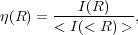
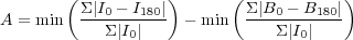
I give a brief description for how these parameters are measured. Typically, as we discuss below, corrections must be applied to account for noise, and to use a reproducible radius (e.g., Bershady et al. 2000; Conselice et al. 2000a). This radius issue has been addressed in detail by e.g., Conselice et al. (2000a), Bershady et al. (2000) and Graham et al. (2005). The radius typically used in these measures is the Petrosian radius, which is defined as the location where the ratio of surface brightness at a radius, I(R), divided by the surface brightness within the radius < I(< R) >, reaches some value, which is denoted by η(R) (Petrosian 1976). The value of η changes from η(0) = 1 at the center of a galaxy, down to η(∞) = 0 when the light from the galaxy is zero at its outer 'edge'.
This method of measuring the radius is much less influenced by surface brightness dimming than other methods such as using an isophotal radius, and is therefore useful for measuring the same physical parts of galaxies at different redshifts (e.g., Petrosian 1976; Bershady et al. 2000; Graham et al. 2005). The mathematical form for this radius is given by
 |
(2) |
where most observables in non-parametric morphologies are measured at a radius which corresponds to the location where η(R) = 0.2, or a relatively small multiplicative factor of this radius (often 1.5 times) (e.g., Bershady et al. 2000; Conselice 2003; Lotz et al. 2004).
2.3.1. ASYMMETRY INDEX One of the more commonly used indices is the asymmetry index(A) which is a measure of how asymmetric a galaxy is after rotating along the line of sight center axis of the galaxy by 180 deg (Figure 2). It can be thought of as an indicator of what fraction of the light in a galaxy is in non-symmetric components.
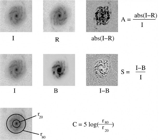 |
Figure 2. A graphical representation of how the concentration (C), asymmetry (A), clumpiness (S) are measured on an example nearby galaxy. Within the measurements for A and S, the value 'I' represents the original galaxy image, while 'R' is this image rotated by 180 deg. For the clumpiness S, 'B' is the image after it has been smoothed (blurred) by the factor 0.3 × r(η = 0.2). The details of these measurements can be found in Conselice et al. (2000a) for asymmetry, A, Bershady et al. (2000) for concentration, C, and Conselice (2003) for the clumpiness index, S. |
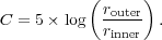
The basic formula for calculating the asymmetry index (A) is given by:
 |
(3) |
Where I0 represents is the original galaxy image, I180 is the image after rotating it from its center by 180°. The measurement of the asymmetry parameter however involves several steps beyond this simple measure. This includes carefully dealing with the background noise in the same way that the galaxy itself is by using a blank background area (B0), and finding the location for the center of rotation. The radius is usually defined as the Petrosian radius at which η(R) = 0.2, although once out to large radius the measured parameters are remarkably stable.
Operationally, the area B0 is a blank part of the sky near the galaxy. The center of rotation is not defined a priori, but is measured through an iterative process whereby the value of the asymmetry is calculated at the initial central guess (usually the geometric center or light centroid) and then the asymmetry is calculated around this central guess using some fraction of a pixel difference. This is repeated until a global minimum is found (Conselice et al. 2000a).
Typical asymmetry values for nearby galaxies are discussed in Conselice (2003) with ellipticals having values A ~ 0.02 ± 0.02, while spiral galaxies are found in the range from A ~ 0.07-0.2, while for Ultra-Luminous Infrared Galaxies (ULIRGs), which are often mergers, the average is A ~ 0.32 ± 0.19, and for merging starbursts A ~ 0.53 ± 0.22 (Conselice 2003). Table 1 lists the typical asymmetry and other CAS values (Conselice 2003). Quantitative structural values for the same galaxy can also differ significantly between wavelengths. This is important for measuring these parameters at higher redshifts, where often the rest-frame optical cannot be probed, an issue we discuss in more detail in Section 2.3.5.
| Galaxy Type | Concentration (R) | Asymmetry (A) | clumpiness (C) |
| Ellipticals | 4.4 ± 0.3 | 0.02 ± 0.02 | 0.00 ± 0.04 |
| Early-type disks (Sa-Sb) | 3.9 ± 0.5 | 0.07 ± 0.04 | 0.08 ± 0.08 |
| Late-type disks (Sc-Sd) | 3.1 ± 0.4 | 0.15 ± 0.06 | 0.29 ± 0.13 |
| Irregulars | 2.9 ± 0.3 | 0.17 ± 0.10 | 0.40 ± 0.20 |
| Edge-on Disks | 3.7 ± 0.6 | 0.17 ± 0.11 | 0.45 ± 0.20 |
| ULIRGs | 3.5 ± 0.7 | 0.32 ± 0.19 | 0.50 ± 0.40 |
| Starbursts | 2.7 ± 0.2 | 0.53 ± 0.22 | 0.74 ± 0.25 |
| Dwarf Ellipticals | 2.5 ± 0.3 | 0.02 ± 0.03 | 0.00 ± 0.06 |
2.3.2. LIGHT CONCENTRATION The concentration of light is used as a method for quantifying how much light is in the center of a galaxy as opposed to its outer parts. It is a very simple index in this regard, and it is similar to, and correlates strongly with, Sérsic n values, which are also a measure of the light concentration in a galaxy. There are many ways of measuring the concentration, including taking ratios of radii which contain a certain fraction of light, as well as the ratio of the amount of light at two given radii (e.g., Bershady et al. 2000; Graham et al. 2005). These radii are often defined by the total amount of light measured within some Petrosian radius, often at the same location as used for the measuring the asymmetry index.
The definition most commonly used is the ratio of two circular radii which contain a inner and outer fraction (20% and 80% or 30% and 70% are the most common) (rinner, router) of the total galaxy flux (Figure 2),
 |
(4) |
A higher value of C indicates that a larger amount of light in a galaxy is contained within a central region. The concentration index however has to be measured very carefully, as different regions and radii used can produce very different values that systematically do not reproduce well when observed under degraded conditions (e.g., Graham et al. 2001; Graham et al. 2005).
2.3.3. CLUMPINESS The clumpiness (or smoothness) (S) parameter is used to describe the fraction of light in a galaxy which is contained in clumpy distributions. Clumpy galaxies have a relatively large amount of light at high spatial frequencies, whereas smooth systems, such as elliptical galaxies contain light at low spatial frequencies. Galaxies which are undergoing star formation tend to have very clumpy structures, and thus high S values. Clumpiness can be measured in a number of ways, the most common method used, as described in Conselice (2003) is,
 |
(5) |
where, the original image Ix,y is blurred to produce a secondary image, Ix,yσ (Figure 2). This blurred image is then subtracted from the original image leaving a residual map, containing only high frequency structures in the galaxy (Conselice 2003). The size of the smoothing kernel σ is determined by the radius of the galaxy, and the value σ = 0.2 ⋅ 1.5 × r(η = 0.2) gives the best signal for nearby systems (Conselice 2003). Note that the centers of galaxies are removed when this procedure is carried out as they often contain unresolved high-spatial frequency light.
Figure 3 shows a diagram for how these three CAS parameters are measured on a typical nearby spiral galaxy. Furthermore, the CAS parameters can be combined together to create a 3-dimension space in which different galaxy types can be classified. For example, Figure 3 shows the concentration vs. asymmetry vs. clumpiness diagram, demonstrating how these parameters can be used to determine morphological types of galaxies in the nearby universe in CAS space.
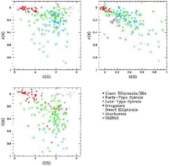 |
Figure 3. The different forms of the realizations of nearby galaxies of different morphologies and evolutionary states plotted together in terms of their CAS parameters. The top left panel shows the concentration and asymmetry indexes plotted with colored points that reflect the value of the clumpiness for each galaxy. Systems that have clumpiness values, S < 0.1 are colored red, galaxies with values 0.1 < S < 0.35 are green, and systems with S > 0.35 are blue. In a similar way for the A-S diagram: red are for galaxies with for C > 4, green for systems with 3 < C < 4, and blue points for C < 3. For the S-C diagram: red is for systems with asymmetries A < 0.1, green have values 0.1 < A < 0.35, and blue for A > 0.35. When using these three morphological parameters all known nearby galaxy types can be distinctly separated and distinguished in structural space (Conselice 2003). |
2.3.4. OTHER COEFFICIENTS Another popular structural measurement system is the Gini/M20 parameters which are used in a similar way to the CAS parameters to find galaxies of broad morphological types, especially galaxies undergoing mergers (e.g., Abraham et al. 2003; Lotz et al. 2004). Both of these parameters measure the relative distribution of light within pixels, and do not involve subtraction, as is used for the asymmetry and clumpiness parameters, and therefore in principle may be less sensitive to high levels of background noise (e.g., Lotz et al. 2004).
The Gini coefficient is a statistical tool originally used in economics to determine the distribution of wealth within a population, with higher values indicating a very unequal distribution (Gini of 1 would mean all wealth/light is in one person/pixel), while a lower value indicates it is distributed more evenly amongst the population (Gini of 0 would mean everyone/every pixel has an equal share). The value of G is defined by the Lorentz curve of the galaxy's light distribution, which does not take into consideration spatial position.
In the calculation of these parameters, each pixel is ordered by its brightness and counted as part of the cumulative distribution (see Lotz et al. 2004, 2008). A galaxy in this case is considered a system with n pixels each with a flux fi where i ranges from 0 to n. The Gini coefficient is then measured by
 |
(6) |
where
 is the
average pixel flux value. The second
order moment parameter, M20,
is similar to the concentration in that it gives a value that indicates
whether light is concentrated within an image.
However a M20 value denoting a high concentration (a very
negative value) does not imply a central concentration, as in principle
the light could be concentrated
in any location in a galaxy. The value of M20 is the moment
of the fluxes of the brightest 20% of light in a galaxy, which is
then normalized by the total light moment for all pixels
(Lotz et al. 2004,
2008).
The mathematical form for the M20 index is
is the
average pixel flux value. The second
order moment parameter, M20,
is similar to the concentration in that it gives a value that indicates
whether light is concentrated within an image.
However a M20 value denoting a high concentration (a very
negative value) does not imply a central concentration, as in principle
the light could be concentrated
in any location in a galaxy. The value of M20 is the moment
of the fluxes of the brightest 20% of light in a galaxy, which is
then normalized by the total light moment for all pixels
(Lotz et al. 2004,
2008).
The mathematical form for the M20 index is
 |
(7) |
where the value of Mtot is
 |
where xc and yc is the center of galaxy, which in the case of M20 this center is defined as the location where the value of Mtot is minimized (Lotz et al 2004). The separation for nearby elliptical, spirals and ULIRGs is similar to that found by the CAS parameters (see Lotz et al. 2004, 2008).
Other popular parameters include the multiplicity index, Ψ, which is a measure of the potential energy of a light distribution (e.g., Law et al. 2007). Values of Ψ range from 0 for systems that are in the most compact forms, to those with values Ψ > 10 which are often very irregular/peculiar (e.g., Law et al. 2012a). Another recent suite of parameters developed by Freeman et al. (2013) include features that measure the multi-mode (M), intensity (I), and deviation (D) of a galaxy's light profile with the intention to locate galaxy mergers.
2.3.5. REDSHIFT EFFECTS ON STRUCTURE One of the major issues with non-parametric structural indices is that they will change for more distant galaxies, both due to any evolution but also due to distance effects, creating a smaller and fainter image of the same system. This must be accounted for when using galaxy structure as a measure of evolution (e.g., Conselice et al. 2000a; Conselice 2003; Lisker 2008).
There are several ways to deal with this issue, which is similar to how corrections for point spread functions in parametric fitting or weak lensing analyses are done. The most common correction method for non-parametric parameters is to use image simulations. These simulations are such that nearby galaxies are reduced in resolution and surface brightness to match the redshift at which the galaxy is to be simulated at. These new simulated images are then placed into a background appropriate for the instrument and exposure time in which the simulation takes place (Conselice 2003). The outline for how to do these simulations is provided in papers such as Giavalisco et al. (1996) and Conselice (2003) amongst others.
To give some idea of the difficultly in reproducing the morphologies and structures of galaxies, Figure 4 shows simulated nearby early-type spirals as to how they would appear in WFC3 imaging data from the Hubble Ultra Deep Field (Conselice et al. 2011a). What can be clearly seen is that it is difficult, and sometimes even impossible, to make out features of these galaxies after they have been simulated.
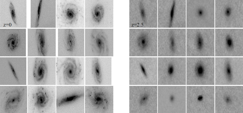 |
Figure 4. Nearby galaxies originally observed at z ~ 0 in the rest-frame B-band simulated to how they would appear at z = 2.5, also observed in the rest-frame B-band, within the Hubble Ultra Deep Field WFC3 F160W (H) band. These systems are classified as late-type spirals (Sc and Sd) in the nearby universe but can appear very different when simulated to higher redshifts as can be seen here and when using quantitative measures. The typical sizes of these galaxies are several kpc in effective radii, and are at a variety of distances (see Conselice et al. 2000a, Conselice et al. 2011a). These changes in structure, both in apparent morphology and in terms of the structural indices must be carefully considered before evolution is derived (e.g., Conselice et al. 2008; Mortlock et al. 2013). |
Another issue when examining the structures of distant galaxies is that these systems will often be observed at bluer wavelengths than what is typically observed with in the nearby universe due to the effects of redshift. For example, pictures of galaxies at z > 1.2 taken with WFPC2 and ACS are all imaged in the rest-frame ultraviolet. Figure 5 shows what rest-frame wavelength various popular filters probe as a function of redshift. This shows that we must go to the near infrared to probe rest-frame optical light for galaxies at z > 1.
 |
Figure 5. Plot showing the rest-frame wavelength probed by the most common filters used to image distant galaxies as a function of redshift from z ~ 0-6. The filters shown are the ACS B450, V550, i775, z950 filters, and the WFC3 J110 and H160 filters and a K-band filter centered at 2.2 μm. The shaded area shows the region in which the rest-frame optical light of distant galaxies can be probed from between 0.38 μm to 0.9 μm. As can be seen, the H-band allows rest-frame light up to z ~ 3 to be imaged, while the K-band can extend this out to z ~ 4.5. |
It turns out that the qualitative and quantitative morphologies and structures of galaxies can vary significantly between rest-frame ultraviolet and rest-frame optical images (e.g., Meurer et al. 1995; Hibbard & Vacca 1997; Windhorst et al. 2002; Taylor-Mager et al. 2007) although these morphologies are not significantly different for starbursting galaxies with little dust at both low and high redshift (Dickinson 2000; Conselice et al. 2000b). While it is clear that the CAS method works better at distinguishing types at redder wavelengths (e.g., Lanyon-Foster et al. 2012), its use has also expanded into image analyses with HI and dust-emission maps from Spitzer (e.g., Bendo et al. 2007; Holwerda et al. 2011, 2013).
The process for accounting for the effects of image degradation is to measure the morphological index of interest at z = 0, and then to remeasure the same values at higher redshift after simulating. For the morphological k-correction the approach has been to measure the parameter of interest at different wavelengths, and to determine by interpolation the value at the rest-frame wavelength of interest.
Using the asymmetry index as an example, the final measure after correcting for redshift effects is,
 |
(8) |
where δ Ak<-corr is the (usually negative) morphological k-correction, δ ASB-dim is the (positive) correction for images degradation effects. Other parameters can be measured the same way. This is a necessary correction to examine the evolution of a selected population at the same effective depth, resolution and rest-frame wavelength.