


Equation 1 was first used by Lanzetta et al. (1995) to study the chemical evolution of the damped Lyα absorption systems, where one infers the comoving rate of star formation from the observed cosmological mass density of H I. Pei & Fall (1995) then generalized it to models with inflows and outflows. Madau et al. (1996, 1998b) and Lilly et al. (1996) developed a different method where data from galaxy surveys were used to infer the SFRD ψ(t) directly. This new approach relies on coupling the equations of chemical evolution to the spectrophotometric properties of the cosmic volume under consideration. The specific luminosity density at time t of a "cosmic stellar population" characterized by an SFRD ψ(t) and a metal-enrichment law Z∗(t) is given by the convolution integral
 |
(13) |
where  ν[τ,
Z∗(t - τ)] is the specific
luminosity density radiated per unit initial stellar mass by
a SSP of age τ and metallicity Z∗(t
- τ). The theoretical calculation of
ν requires
stellar evolutionary tracks, isochrones, and stellar atmosphere
libraries. As an illustrative example of this technique, we provide in
this section a current determination of the SFH of the Universe and
discuss a number of possible implications.
ν[τ,
Z∗(t - τ)] is the specific
luminosity density radiated per unit initial stellar mass by
a SSP of age τ and metallicity Z∗(t
- τ). The theoretical calculation of
ν requires
stellar evolutionary tracks, isochrones, and stellar atmosphere
libraries. As an illustrative example of this technique, we provide in
this section a current determination of the SFH of the Universe and
discuss a number of possible implications.
Rather than trying to be exhaustive, we base our modeling below on a limited number of contemporary (mostly post-2006) galaxy surveys (see Table 1). For the present purpose, we consider only surveys that have measured SFRs from rest-frame FUV (generally 1,500 Å) or MIR and FIR measurements. Other surveys of nebular line or radio emission are also important, but they provide more limited or indirect information as discussed in previous sections (Sections 4.3 and 4.4). For the IR measurements, we emphasize surveys that make use of FIR data from Spitzer or Herschel, rather than relying on MIR (e.g., Spitzer 24-μm) measurements alone, owing to the complexity and lingering uncertainty over the best conversions from MIR luminosity to SFR, particularly at high redshift or high luminosity. In a few cases, we include older measurements when they are the best available, particularly for local luminosity densities from IRAS or GALEX, or GALEX-based measurements at higher redshifts that have not been updated since 2005.
| Reference | Redshift range | AFUVa | logψb | Symbols used in Figure 9 | |
| [mag] | [M⊙ year-1 Mpc-3] | ||||
| Wyder et al. (2005) | 0.01-0.1 | 1.80 | -1.82-0.02+0.09 | blue-gray hexagon | |
| Schiminovich et al. (2005) | 0.2-0.4 | 1.80 | -1.50-0.05+0.05 | blue triangles | |
| 0.4-0.6 | 1.80 | -1.39-0.08+0.15 | |||
| 0.6-0.8 | 1.80 | -1.20-0.13+0.31 | |||
| 0.8-1.2 | 1.80 | -1.25-0.13+0.31 | |||
| Robotham & Driver (2011) | 0.05 | 1.57 | -1.77-0.09+0.08 | dark green pentagon | |
| Cucciati et al. (2012) | 0.05-0.2 | 1.11 | -1.75-0.18+0.18 | green squares | |
| 0.2-0.4 | 1.35 | -1.55-0.12+0.12 | |||
| 0.4-0.6 | 1.64 | -1.44-0.10+0.10 | |||
| 0.6-0.8 | 1.92 | -1.24-0.10+0.10 | |||
| 0.8-1.0 | 2.22 | -0.99-0.08+0.09 | |||
| 1.0-1.2 | 2.21 | -0.94-0.09+0.09 | |||
| 1.2-1.7 | 2.17 | -0.95-0.08+0.15 | |||
| 1.7-2.5 | 1.94 | -0.75-0.09+0.49 | |||
| 2.5-3.5 | 1.47 | -1.04-0.15+0.26 | |||
| 3.5-4.5 | 0.97 | -1.69-0.32+0.22 | |||
| Dahlen et al. (2007) | 0.92-1.33 | 2.03 | -1.02-0.08+0.08 | turquoise pentagons | |
| 1.62-1.88 | 2.03 | -0.75-0.12+0.12 | |||
| 2.08-2.37 | 2.03 | -0.87-0.09+0.09 | |||
| Reddy & Steidel (2009) | 1.9-2.7 | 1.36 | -0.75-0.11+0.09 | dark green triangles | |
| 2.7-3.4 | 1.07 | -0.97-0.15+0.11 | |||
| Bouwens et al. (2012a), (2012b) | 3.8 | 0.58 | -1.29-0.05+0.05 | magenta pentagons | |
| 4.9 | 0.44 | -1.42-0.06+0.06 | |||
| 5.9 | 0.20 | -1.65-0.08+0.08 | |||
| 7.0 | 0.10 | -1.79-0.10+0.10 | |||
| 7.9 | 0.0 | -2.09-0.11+0.11 | |||
| Schenker et al. (2013) | 7.0 | 0.10 | -2.00-0.11+0.10 | black crosses | |
| 8.0 | 0.0 | -2.21-0.14+0.14 | |||
| Sanders et al. (2003) | 0.03 | — | -1.72-0.03+0.02 | brown circle | |
| Takeuchi et al. (2003) | 0.03 | — | -1.95-0.20+0.20 | dark orange square | |
| Magnelli et al. (2011) | 0.40-0.70 | — | -1.34-0.11+0.22 | red open hexagons | |
| 0.70-1.00 | — | -0.96-0.19+0.15 | |||
| 1.00-1.30 | — | -0.89-0.21+0.27 | |||
| 1.30-1.80 | — | -0.91-0.21+0.17 | |||
| 1.80-2.30 | — | -0.89-0.25+0.21 | |||
| Magnelli et al. (2013) | 0.40-0.70 | — | -1.22-0.11+0.08 | red filled hexagons | |
| 0.70-1.00 | — | -1.10-0.13+0.10 | |||
| 1.00-1.30 | — | -0.96-0.20+0.13 | |||
| 1.30-1.80 | — | -0.94-0.18+0.13 | |||
| 1.80-2.30 | — | -0.80-0.15+0.18 | |||
| Gruppioni et al. (2013) | 0.00-0.30 | — | -1.64-0.11+0.09 | dark red filled hexagons | |
| 0.30-0.45 | — | -1.42-0.04+0.03 | |||
| 0.45-0.60 | — | -1.32-0.05+0.05 | |||
| 0.60-0.80 | — | -1.14-0.06+0.06 | |||
| 0.80-1.00 | — | -0.94-0.06+0.05 | |||
| 1.00-1.20 | — | -0.81-0.05+0.04 | |||
| 1.20-1.70 | — | -0.84-0.04+0.04 | |||
| 1.70-2.00 | — | -0.86-0.03+0.02 | |||
| 2.00-2.50 | — | -0.91-0.12+0.09 | |||
| 2.50-3.00 | — | -0.86-0.23+0.15 | |||
| 3.00-4.20 | — | -1.36-0.50+0.23 | |||
| a In our notation, AFUV ≡ -2.5log10 < kd>. | |||||
| b All our star-formation rate densities are based on the integration of the best-fit luminosity function parameters down to the same relative limiting luminosity, in units of the characteristic luminosity L∗, of Lmin = 0.03 L∗. A Salpeter initial mass function has been assumed. | |||||
For rest-frame FUV data, we use local GALEX measurements by
Wyder et al. (2005)
and
Robotham & Driver
(2011)
and also include the 1,500-Å GALEX measurements at z < 1
from
Schiminovich et
al. (2005).
We use the FUV luminosity densities of
Cucciati et al. (2012)
at 0.1 < z < 4, noting that for z < 1
these are extrapolations from photometry at longer UV rest-frame
wavelengths. At 1
 z
3)
we also use FUV luminosity densities from
Dahlen et al. (2007)
and
Reddy & Steidel
(2009).
At redshifts 4 ≤ z ≤ 8, there are a plethora of
HST-based studies, with some groups of authors
repeatedly re-analyzing samples in GOODS and the HUDF as new and
improved data have accumulated. We restrict our choices to a few of the
most recent analyses, taking best-fit Schechter parameters
(ϕ∗, L∗, α) from
Bouwens et al. (2012b)
and
Schenker et al. (2013).
For the present analysis, we stop at z = 8 and do not consider
estimates at higher redshifts.
z
3)
we also use FUV luminosity densities from
Dahlen et al. (2007)
and
Reddy & Steidel
(2009).
At redshifts 4 ≤ z ≤ 8, there are a plethora of
HST-based studies, with some groups of authors
repeatedly re-analyzing samples in GOODS and the HUDF as new and
improved data have accumulated. We restrict our choices to a few of the
most recent analyses, taking best-fit Schechter parameters
(ϕ∗, L∗, α) from
Bouwens et al. (2012b)
and
Schenker et al. (2013).
For the present analysis, we stop at z = 8 and do not consider
estimates at higher redshifts.
For local IR estimates of the SFRD, we use IRAS LFs from Sanders et al. (2003) and Takeuchi et al. (2003). At 0.4 < z < 2.3, we include data from Magnelli et al. (2009, 2011), who used stacked Spitzer 70-μm measurements for 24-μm-selected sources. We also use the Herschel FIRLFs of Gruppioni et al. (2013) and Magnelli et al. (2013). Although both groups analyze data from the GOODS fields, Gruppioni et al. (2013) incorporate wider/shallower data from COSMOS. By contrast, Magnelli et al. (2013) include the deepest 100- and 160-μm data from GOODS-Herschel, extracting sources down to the faintest limits using 24-μm prior positions.
All the surveys used here provide best-fit LF parameters - generally Schechter functions for the UV data, but other functions for the IR measurements, such as double power laws or the function by Saunders et al. (1990). These allow us to integrate the LF down to the same relative limiting luminosity, in units of the characteristic luminosity L∗. We adopt an integration limit Lmin = 0.03 L∗ when computing the luminosity density ρFUV or ρIR. For the case of a Schechter function, this integral is
 |
(14) |
Here α denotes the faint-end slope of the Schechter
parameterization, and Γ is the incomplete gamma function. The
integrated luminosity density has a strong dependence on
Lmin at high redshift, where the faint-end slope is
measured to be very steep, i.e., α = -2.01 ± 0.21 at z
~ 7 and α = -1.91 ± 0.32 at z ~ 8
(Bouwens et al. 2011b).
Slopes of α
-2 lead to formally divergent luminosity densities. Our choice of a
limiting luminosity that is 3.8 magnitudes fainter than
L∗, although it samples a significant portion
of the faint-end of the FUV LF, requires only a mild extrapolation (1.3
mag) from the deepest HST WFC3/IR observations (~ 2.5 mag beyond
L∗ at z ~ 5-8) of the HUDF
(Bouwens et al. 2011b).
For the IR data, we use analytic or numerical integrations
depending on the LF form adopted by each reference, but the same
faint-end slope considerations apply. (Note, however, that some authors
use logarithmic slopes for IRLFs, which differ from the linear form used
in the standard Schechter formula by Δ α = +1.)
Multiplying the integrated FUV and IR comoving luminosity densities by
the conversion factors
 FUV
(Section 3.1.1) and
IR
(Section 3.1.2),
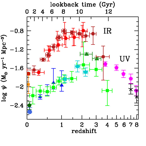
we obtain measurements of the "observed" UV and IR SFRDs (shown in
Figure 8). Here, the FUV measurements are
uncorrected for dust attenuation. This illustrates the now well-known
result that most of the energy from star-forming galaxies
at 0 < z < 2 is absorbed and reradiated by dust; only a
minority fraction emerges directly from galaxies as UV light. The gap
between the UV and IR measurements increases with
redshift out to at least z ≈ 1 and then may narrow from
z = 1 to 2. Robust measurements of the FIR luminosity density are
not yet available at z > 2.5.
FUV
(Section 3.1.1) and
IR
(Section 3.1.2),
we obtain measurements of the "observed" UV and IR SFRDs (shown in
Figure 8). Here, the FUV measurements are
uncorrected for dust attenuation. This illustrates the now well-known
result that most of the energy from star-forming galaxies
at 0 < z < 2 is absorbed and reradiated by dust; only a
minority fraction emerges directly from galaxies as UV light. The gap
between the UV and IR measurements increases with
redshift out to at least z ≈ 1 and then may narrow from
z = 1 to 2. Robust measurements of the FIR luminosity density are
not yet available at z > 2.5.
 |
 |
Figure 8. (Left panel) SFR
densities in the FUV (uncorrected for dust attenuation) and in the FIR.
The data points with symbols are given in
Table 1. All UV and IR
luminosities have been converted to
instantaneous SFR densities using the factors
|
|
Clearly, a robust determination of dust attenuation is essential to transform FUV luminosity densities into total SFRDs. Figure 8 shows measurements of the effective dust extinction, < kd >, as a function of redshift. This is the multiplicative factor needed to correct the observed FUV luminosity density to the intrinsic value before extinction, or equivalently, < kd > = ρIR / ρFUV + 1 (e.g., Meurer et al. 1999). For most of the data shown in Figure 8, the attenuation has been estimated from the UV spectral slopes of star-forming galaxies using the attenuation-reddening relations from Meurer et al. (1999) or Calzetti et al. (2000) or occasionally from stellar population model fitting to the full UV-optical SEDs of galaxies integrated over the observed population (e.g., Salim et al. 2007, Cucciati et al. 2012). Robotham & Driver (2011) used the empirical attenuation correction of Driver et al. (2008). We note that the estimates of UV attenuation in the local Universe span a broad range, suggesting that more work needs to be done to firmly pin down this quantity (and perhaps implying that we should be cautious about the estimates at higher redshift). Several studies of UV-selected galaxies at z ≥ 2 (Reddy & Steidel 2009, Bouwens et al. 2012a, Finkelstein et al. 2012b) have noted strong trends for less luminous galaxies as having bluer UV spectral slopes and, hence, lower inferred dust attenuation. Because the faint-end slope of the far-UV luminosity function (FUVLF) is so steep at high redshift, a large fraction of the reddened FUV luminosity density is emitted by galaxies much fainter than L∗; this extinction-luminosity trend also implies that the net extinction for the entire population will be a function of the faint integration limit for the sample. In Figure 8, the points from Reddy & Steidel (2009) (at z = 2.3 and 3.05) and from Bouwens et al. (2012a) (at 2.5 ≤ z ≤ 7) are shown for two faint-end integration limits: These are roughly down to the observed faint limit of the data, MFUV < -17.5 to -17.7 for the different redshift subsamples and extrapolated to LFUV = 0. The net attenuation for the brighter limit, which more closely represents the sample of galaxies actually observed in the study, is significantly larger than for the extrapolation - nearly two times larger for the Reddy & Steidel (2009) samples, and by a lesser factor for the more distant objects from Bouwens et al. (2012a). In our analysis of the SFRDs, we have adopted the mean extinction factors inferred by each survey to correct the corresponding FUV luminosity densities.
Adopting a different approach, Burgarella et al. (2013) measured total UV attenuation from the ratio of FIR to observed (uncorrected) FUV luminosity densities (Figure 8) as a function of redshift, using FUVLFs from Cucciati et al. (2012) and Herschel FIRLFs from Gruppioni et al. (2013). At z < 2, these estimates agree reasonably well with the measurements inferred from the UV slope or from SED fitting. At z > 2, the FIR/FUV estimates have large uncertainties owing to the similarly large uncertainties required to extrapolate the observed FIRLF to a total luminosity density. The values are larger than those for the UV-selected surveys, particularly when compared with the UV values extrapolated to very faint luminosities. Although galaxies with lower SFRs may have reduced extinction, purely UV-selected samples at high redshift may also be biased against dusty star-forming galaxies. As we noted above, a robust census for star-forming galaxies at z ≫ 2 selected on the basis of dust emission alone does not exist, owing to the sensitivity limits of past and present FIR and submillimeter observatories. Accordingly, the total amount of star formation that is missed from UV surveys at such high redshifts remains uncertain.
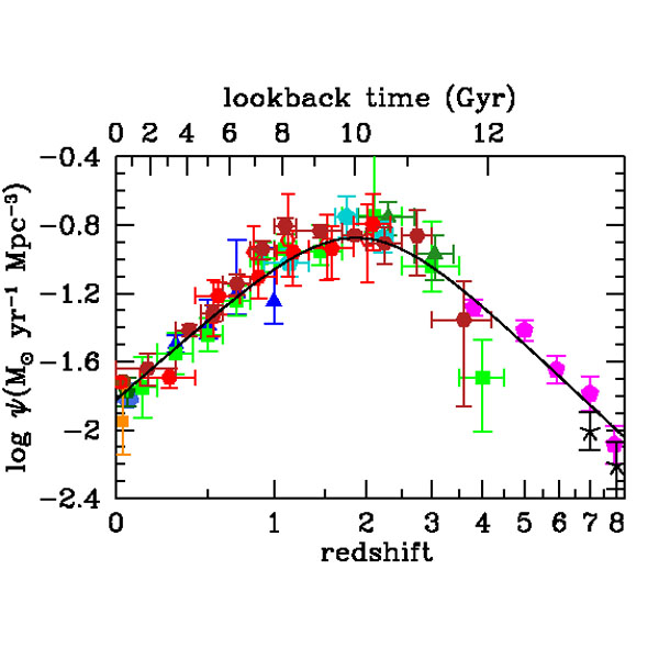
Figure 9 shows the cosmic SFH from UV and IR data following the above prescriptions, as well as the best-fitting function
 |
(15) |
These state-of-the-art surveys provide a remarkably consistent picture
of the cosmic SFH:
a rising phase, scaling as ψ(z) ∝ (1 +
z)-2.9 at 3
z
8, slowing and
peaking at some point probably between z = 2 and 1.5, when the
Universe was ~ 3.5 Gyr old, followed by a gradual
decline to the present day, roughly as ψ(z) ∝ (1 +
z)2.7. The comoving SFRD at redshift 7 was
approximately the same as that measured locally. The increase in
ψ(z) from z ≈ 8 to 3 appears to have
been steady, with no sharp drop at the highest redshifts, although there
is now active debate in the literature about whether that trend
continues or breaks at redshifts 9 and beyond
(Coe et al. 2013,
Ellis et al. 2013,
Oesch et al. 2013).
Although we have adopted a fitting function that is a double power-law
in (1 + z), we note that the SFRD data at z < 1
can also be fit quite well by an exponential decline with cosmic time
and an e-folding timescale of 3.9 Gyr. Compared with
the recent empirical fit to the SFRD by
Behroozi et al. (2013),
the function in Equation 15 reaches its
peak at a slightly higher redshift, with a lower maximum value of ψ
and with slightly shallower rates of change at both
lower and higher redshift, and produces 20% fewer stars by z = 0.
 |
 |
Figure 9. The history of cosmic star
formation from (top right panel) FUV, (bottom right panel) IR, and
(left panel) FUV+IR rest-frame measurements. The data points with
symbols are given in Table 1.
All UV luminosities have been converted to instantaneous SFR densities
using the factor
|
|
We also note that each published measurement has its own approach to computing uncertainties on the SFRD and takes different random and systematic factors into account, and we have made no attempt to rationalize these here. Moreover, the published studies integrate their measurements down to different luminosity limits. We have instead adopted a fixed threshold of 0.03 L∗ to integrate the published LFs, and given the covariance on the measurements and uncertainties of LF parameters, there is no simple way for us to correct the published uncertainties to be appropriate for our adopted integration limit. Therefore, we have simply retained the fractional errors on the SFRD measurements published by each author without modification to provide an indication of the relative inaccuracy derived by each study. These should not be taken too literally, especially when there is significant difference in the faint-end slopes of LFs reported in different studies, which can lead to large differences in the integrated luminosity density. Uncertainties in the faint-end slope and the resulting extrapolations are not always fully taken into account in published error analyses, especially when LFs are fit at high redshift by fixing the slope to some value measured only at lower redshift.
5.2. Core-Collapse Supernova Rate
Because core-collapse supernovae (CC SNe) (i.e., Type II and Ibc SNe) originate from massive, short-lived stars, the rates of these events should reflect ongoing star formation and offer an independent determination of the cosmic star formation and metal production rates at different cosmological epochs (e.g., Madau et al. 1998a, Dahlen et al. 2004). While poor statistics and dust obscuration are major liming factors for using CC SNe as a tracer of the SFH of the Universe, most derived rates are consistent with each other and increase with lookback time between z = 0 and z ~ 1 (see Figure 10). The comoving volumetric SN rate is determined by multiplying Equation 15 by the efficiency of forming CC SNe
 |
(16) |
where the number of stars that explode as SNe per unit mass is kCC = 0.0068 M⊙-1 for a Salpeter IMF, mmin = 8 M⊙, and mmax = 40 M⊙. The predicted cosmic SN rate is shown in Figure 10 and appears to be in good agreement with the data. The IMF dependence in Equation 16 is largely canceled out by the IMF dependence of the derived SFRD ψ(z), as the stellar mass range probed by SFR indicators is comparable to the mass range of stars exploding as CC SNe. Recent comparisons between SFRs and CC SN rates have suggested a discrepancy between the two rates: The numbers of CC SNe detected are too low by a factor of approximately (Horiuchi et al. 2011). Our revised cosmic SFH does not appear to show such systematic discrepancy (see also Dahlen et al. 2012).
 |
Figure 10. The cosmic core-collapse SN rate. The data points are taken from Li et al. (2011) (cyan triangle), Mattila et al. (2012) (red dot), Botticella et al. (2008) (magenta triangle), Bazin et al. (2009) (gray square), and Dahlen et al. (2012) (blue dots). The solid line shows the rates predicted from our fit to the cosmic star-formation history. The local overdensity in star formation may boost the local rate within 10-15 Mpc of Mattila et al. (2012). |
Observations show that at least some long-duration gamma-ray bursts (GRBs) happen simultaneously with CC SNe, but neither all SNe, nor even all SNe of Type Ibc produce GRBs (for a review, see Woosley & Bloom 2006). In principle, the rate of GRBs of this class could provide a complementary estimate of the SFRD (e.g., Porciani & Madau 2001), but it is only a small fraction (< 1% after correction for beaming) of the CC SN rate (Gal-Yam et al. 2006), suggesting that GRBs are an uncommon chapter in the evolution of massive stars requiring special conditions that are difficult to model. Recent studies of the GRB-SFR connection have claimed that GRBs do not trace the SFR in an unbiased way, and are more frequent per unit stellar mass formed at early times (Kistler et al. 2009, Robertson & Ellis 2012, Trenti et al. 2012).
Figure 11 shows a compilation (see also
Table 2) of recent (mostly post 2006)
measurements of
the SMD as a function of redshift (for a compilation of older data see
Wilkins et al. 2008a).
We show local SDSS-based SMDs from
Gallazzi et al. (2008),
Li & White (2009),
and
Moustakas et al. (2013).
Moustakas et al. (2013)
also measured SMFs at 0.2 < z < 1. However, at z
> 0.5 their mass completeness limit is
larger than 109.5 M⊙, so we have used
their points only below that redshift. At higher redshifts (as in
Moustakas et al. 2013),
nearly all the modern estimates incorporate Spitzer IRAC photometry;
we include only one recent analysis
(Bielby et al. 2012)
that does not but that otherwise uses excellent deep, wide-field NIR
data in four independent sightlines. We also include measurements at 0.1
< z 4
from
Arnouts et al. (2007),
Pérez-González et
al. (2008),
Kajisawa et al. (2009),
Marchesini et al. (2009),
Reddy & Steidel
(2009),
Pozzetti et al. (2010),
Ilbert et al. (2013),
and
Muzzin et al. (2013).
We show measurements for the IRAC-selected sample of
Caputi et al. (2011)
at 3 ≤ z ≤ 5 and for
UV-selected LBG samples at 4 < z < 8 by
Yabe et al. (2009),
González et
al. (2011),
Lee et al. (2012),
and
Labbé et al. (2013).
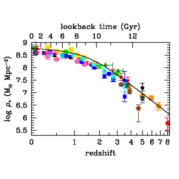 |
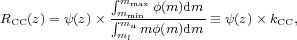
Figure 11. The evolution of the stellar mass density. The data points with symbols are given in Table 2. The solid line shows the global stellar mass density obtained by integrating the best-fit instantaneous star-formation rate density ψ(z) (Equations 2 and 15) with a return fraction R = 0.27. |
When needed, we have scaled from a Chabrier IMF to a Salpeter IMF by multiplying the stellar masses by a factor of 1.64 (Figure 4). At high redshift, authors often extrapolate their SMFs beyond the observed range by fitting a Schechter function. Stellar mass completeness at any given redshift is rarely as well defined as luminosity completeness, given the broad range of M / L values that galaxies can exhibit. Unlike the LFs used for the SFRD calculations where we have tried to impose a consistent faint luminosity limit (relative to L∗) for integration, in most cases we have simply accepted whatever low-mass limits or integral values that the various authors reported. Many authors found that the characteristic mass M∗ appears to change little for 0 < z < 3 (e.g., Fontana et al. 2006, Ilbert et al. 2013) and is roughly 1011 M⊙ (Salpeter). Therefore, a low-mass integration limit similar to that which we used for the LFs (Lmin = 0.03 L∗) would correspond to Mmin ≈ 109.5 M⊙ in that redshift range. A common but by no means universal low-mass integration limit used in the literature is 108 M⊙. Generally, SMFs have flatter low-mass slopes than do UVLFs (and sometimes IRLFs), so the lower-mass limit makes less difference to the SMDs than it does to the SFRDs.
| Reference | Redshift range | logρ∗a | Symbols used in Figure 11 | |
| [M⊙ Mpc-3] | ||||
| Li & White (2009) | 0.07 | 8.59-0.01+0.01 | gray dot | |
| Gallazzi et al. (2008) | 0.005-0.22 | 8.78-0.08+0.07 | dark green square | |
| Moustakas et al. (2013) | 0.0-0.2 | 8.59-0.05+0.05 | magenta stars | |
| 0.2-0.3 | 8.56-0.09+0.09 | |||
| 0.3-0.4 | 8.59-0.06+0.06 | |||
| 0.4-0.5 | 8.55-0.08+0.08 | |||
| Bielby et al. (2012) b | 0.2-0.4 | 8.46-0.12+0.09 | pink filled hexagons | |
| 0.4-0.6 | 8.33-0.03+0.03 | |||
| 0.6-0.8 | 8.45-0.1+0.08 | |||
| 0.8-1.0 | 8.42-0.06+0.05 | |||
| 1.0-1.2 | 8.25-0.04+0.04 | |||
| 1.2-1.5 | 8.14-0.06+0.06 | |||
| 1.5-2.0 | 8.16-0.03+0.32 | |||
| Pérez-González et al. (2008) | 0.0-0.2 | 8.75-0.12+0.12 | red triangles | |
| 0.2-0.4 | 8.61-0.06+0.06 | |||
| 0.4-0.6 | 8.57-0.04+0.04 | |||
| 0.6-0.8 | 8.52-0.05+0.05 | |||
| 0.8-1.0 | 8.44-0.05+0.05 | |||
| 1.0-1.3 | 8.35-0.05+0.05 | |||
| 1.3-1.6 | 8.18-0.07+0.07 | |||
| 1.6-2.0 | 8.02-0.07+0.07 | |||
| 2.0-2.5 | 7.87-0.09+0.09 | |||
| 2.5-3.0 | 7.76-0.18+0.18 | |||
| 3.0-3.5 | 7.63-0.14+0.14 | |||
| 3.5-4.0 | 7.49-0.13+0.13 | |||
| Ilbert et al. (2013) | 0.2-0.5 | 8.55-0.09+0.08 | cyan stars | |
| 0.5-0.8 | 8.47-0.08+0.07 | |||
| 0.8-1.1 | 8.50-0.08+0.08 | |||
| 1.1-1.5 | 8.34-0.07+0.10 | |||
| 1.5-2.0 | 8.11-0.06+0.05 | |||
| 2.0-2.5 | 7.87-0.08+0.08 | |||
| 2.5-3.0 | 7.64-0.14+0.15 | |||
| 3.0-4.0 | 7.24-0.20+0.18 | |||
| Muzzin et al. (2013) | 0.2-0.5 | 8.61-0.06+0.06 | blue squares | |
| 0.5-1.0 | 8.46-0.03+0.03 | |||
| 1.0-1.5 | 8.22-0.03+0.03 | |||
| 1.5-2.0 | 7.99-0.03+0.05 | |||
| 2.0-2.5 | 7.63-0.04+0.11 | |||
| 2.5-3.0 | 7.52-0.09+0.13 | |||
| 3.0-4.0 | 6.84-0.20+0.43 | |||
| Arnouts et al. (2007) | 0.3 | 8.78-0.16+0.12 | yellow dots | |
| 0.5 | 8.64-0.11+0.09 | |||
| 0.7 | 8.62-0.10+0.08 | |||
| 0.9 | 8.70-0.15+0.11 | |||
| 1.1 | 8.51-0.11+0.08 | |||
| 1.35 | 8.39-0.13+0.10 | |||
| 1.75 | 8.13-0.13+0.10 | |||
| Pozzetti et al. (2010) | 0.1-0.35 | 8.58 | black squares | |
| 0.35-0.55 | 8.49 | |||
| 0.55-0.75 | 8.50 | |||
| 0.75-1.00 | 8.42 | |||
| Kajisawa et al. (2009) | 0.5-1.0 | 8.63 | green squares | |
| 1.0-1.5 | 8.30 | |||
| 1.5-2.5 | 8.04 | |||
| 2.5-3.5 | 7.74 | |||
| Marchesini et al. (2009) | 1.3-2.0 | 8.11-0.02+0.02 | blue dots | |
| 2.0-3.0 | 7.75-0.04+0.05 | |||
| 3.0-4.0 | 7.47-0.13+0.37 | |||
| Reddy et al. (2012) | 1.9-2.7 | 8.10-0.03+0.03 | dark green triangles | |
| 2.7-3.4 | 7.87-0.03+0.03 | |||
| Caputi et al. (2011) | 3.0-3.5 | 7.32-0.02+0.04 | brown pentagons | |
| 3.5-4.25 | 7.05-0.10+0.11 | |||
| 4.25-5.0 | 6.37-0.54+0.14 | |||
| González et al. (2011)c | 3.8 | 7.24-0.06+0.06 | orange dots | |
| 5.0 | 6.87-0.09+0.08 | |||
| 5.9 | 6.79-0.09+0.09 | |||
| 6.8 | 6.46-0.17+0.14 | |||
| Lee et al. (2012)c | 3.7 | 7.30-0.09+0.07 | gray squares | |
| 5.0 | 6.75-0.16+0.33 | |||
| Yabe et al. (2009) | 5.0 | 7.19-0.35+0.19 | small black pentagon | |
| Labbé et al. (2013) | 8.0 | 5.78-0.30+0.22 | red square | |
| a All the stellar mass densities have been derived assuming a Salpeter initial mass function. | ||||
| b Stellar mass densities were computed by averaging over the four fields studied by Bielby et al. (2012). | ||||
| c Following Stark et al. (2013), the mass densities of González et al. (2011) and Lee et al. (2012) at z ≃ 4, 5, 6, and 7 have been reduced by the factor 1.1, 1.3, 1.6, and 2.4, respectively, to account for contamination by nebular emission lines. | ||||
Our model predicts an SMD that is somewhat high (~ 0.2 dex on average, or 60%) compared with many, but not all, of the data at 0 < z ≲ 3. At 0.2 < z < 2, our model matches the SMD measurements for the Spitzer IRAC-selected sample of Arnouts et al. (2007), but several other modern measurements in this redshift range from COSMOS (Pozzetti et al. 2010, Ilbert et al. 2013, Muzzin et al. 2013) fall below our curve. Carried down to z = 0, our model is somewhat high compared with several, but not all (Gallazzi et al. 2008), local estimates of the SMD (e.g., Cole et al. 2001, Baldry et al. 2008, Li & White 2009).
Several previous analyses (Hopkins & Beacom 2006, but see the erratum; Hopkins & Beacom 2008; Wilkins et al. 2008a) have found that the instantaneous SFH over-predicts the SMD by larger factors, up to 0.6 dex at redshift 3. We find little evidence for such significant discrepancies, although there does appear to be a net offset over a broad redshift range. Although smaller, a ~ 60% effect should not be disregarded. One can imagine several possible causes for this discrepancy; we consider several of them here.
Star formation rates may be overestimated, particularly at high redshift during the peak era of galaxy growth. For UV-based measurements, a likely culprit may be the luminosity-weighted dust corrections, which could be too large, although it is often asserted that UV data are likely to underestimate SFRs in very dusty, luminous galaxies. IR-based SFRs may be overestimated and indeed were overestimated for some high-redshift galaxies in earlier Spitzer studies, although this seems less likely now in the era of deep Herschel FIR measurements. It seems more plausible that the SFRs inferred for individual galaxies may be correct on average but that the luminosity function extrapolations could be too large. Many authors adopt fairly steep (α ≥ -1.6) faint-end slopes to both the UVLFs and IRLFs for distant galaxies. For the UVLFs, the best modern data constrain these slopes quite well, but in the IR current measurements are not deep enough to do so. However, although these extrapolations may be uncertain, the good agreement between the current best estimates of the UV- and IR-based SFRDs at 0 < z < 2.5 (Figure 9) does not clearly point to a problem in either one.
Instead, stellar masses or their integrated SMD may be systematically underestimated. This is not implausible, particularly for star-forming galaxies, where the problem of recent star formation "outshining" older high M / L stars is well known (see Section 5.1). By analyzing mock catalogs of galaxies drawn from simulations with realistic (and complex) SFHs, Pforr et al. (2012) found that the simplifying assumptions that are typically made when modeling stellar masses for real surveys generally lead to systematically underestimated stellar masses at all redshifts. That said, other systematic effects can work in the opposite direction and lead to mass overestimates, e.g., the effects of TP-AGB stars on the red and NIR light if these are not correctly modeled (Maraston 2005). A steeper low-mass slope to the GSMF could also increase the total SMD. This has been suggested even at z = 0, where mass functions have been measured with seemingly great precision and dynamic range (e.g., Baldry et al. 2008). At high redshift, most studies to date have found relatively flat low-mass SMF slopes, but galaxy samples may be incomplete (and photometric redshift estimates poor) for very faint, red, high-M / L galaxies if they exist in significant numbers. Some recent SMF determinations using very deep HST WFC3 observations have found steeper SMF slopes at z > 1.5 (e.g., Santini et al. 2012), and new measurements from extremely deep NIR surveys such as CANDELS are eagerly anticipated. That said, it seems unlikely that the SMF slope at low redshift has been underestimated enough to account for a difference of 0.2 dex in the SMD.
Recent evidence has suggested that strong nebular line emission can significantly affect broadband photometry for galaxies at high redshift, particularly z > 3.8, where Hα (and, at z > 5.3, [OIII]) enter the Spitzer IRAC bands (Shim et al. 2011). Therefore, following Stark et al. (2013), we have divided the SMD of González et al. (2011) at z≃ 4, 5, 6, and 7 in Figure 11 by the factor 1.1, 1.3, 1.6, and 2.4, respectively, to account for this effect. Although considerable uncertainties in these corrections remain, such downward revision to the inferred early SMD improves consistency with expectations from the time-integrated SFRD.
Alternatively, some authors have considered how changing the IMF may help reconcile SMD(z) with the time-integrated SFRD(z) (e.g., Wilkins et al. 2008b). Generally, a more top-heavy or bottom-light IMF will lead to larger luminosities per unit SFR, hence smaller SFR/L conversion factors K (Section 3.1). Mass-to-light ratios for older stellar populations will also tend to be smaller, but not necessarily by the same factor. Although we have used a Salpeter IMF for reference in this review, an IMF with a low-mass turnover (e.g., Chabrier or Kroupa) will yield a larger mass return fraction R and proportionately lower final stellar masses for a given integrated past SFH, by the factor (1 - R1) / (1 - R2) = 0.81, where R1 and R2 = 0.41 and 0.27 for the Chabrier and Salpeter IMFs, respectively (Section 2). The apparent offset between the SMD data and our integrated model ψ(z) can be reduced further to only ~ 0.1 dex without invoking a particularly unusual IMF. Given the remaining potential for systemic uncertainties in the measurements of SFRDs and SMDs, it seems premature to tinker further with the IMF, although if discrepancies remain after further improvements in the measurements and modeling then this topic may be worth revisiting.
In concordance with estimates from the cosmic SFH, the measurements of
the SMD discussed above imply that galaxies formed the bulk
( 75%) of their
stellar
mass at z < 2. Stars formed in galaxies before 11.5 Gyr are
predicted to contribute only 8% of the total stellar mass today. An
important consistency check for all these determinations could come from
studies of the past SFH of the Universe from its present contents. This
"fossil cosmology" approach has benefited from large spectroscopic
surveys in the local Universe such as the 2dFGRS
(Colless et al. 2001)
and the SDSS
(York et al. 2000),
which provide detailed spectral
information for hundreds of thousands of galaxies. Using a sample of
1.7 × 10⁵ galaxies drawn from the SDSS DR2, and
comparing the spectrum of each galaxy to a library of templates by
Bruzual & Charlot
(2003)
(the comparison was based on five spectral
absorption features, namely D4,000, Hβ, and
HδA + HγA as
age-sensitive indexes, and [Mg2Fe] and [MgFe]' as
metal-sensitive indexes),
Gallazzi et al. (2008)
have constructed a
distribution of stellar mass as a function of age (for a similar
analysis on the SDSS DR3 sample, see also
Panter et al. 2007).
In Figure 12, we compare this distribution with
the one predicted by our best-fit cosmic SFH. The latter implies a
mass-weighted mean stellar age,
75%) of their
stellar
mass at z < 2. Stars formed in galaxies before 11.5 Gyr are
predicted to contribute only 8% of the total stellar mass today. An
important consistency check for all these determinations could come from
studies of the past SFH of the Universe from its present contents. This
"fossil cosmology" approach has benefited from large spectroscopic
surveys in the local Universe such as the 2dFGRS
(Colless et al. 2001)
and the SDSS
(York et al. 2000),
which provide detailed spectral
information for hundreds of thousands of galaxies. Using a sample of
1.7 × 10⁵ galaxies drawn from the SDSS DR2, and
comparing the spectrum of each galaxy to a library of templates by
Bruzual & Charlot
(2003)
(the comparison was based on five spectral
absorption features, namely D4,000, Hβ, and
HδA + HγA as
age-sensitive indexes, and [Mg2Fe] and [MgFe]' as
metal-sensitive indexes),
Gallazzi et al. (2008)
have constructed a
distribution of stellar mass as a function of age (for a similar
analysis on the SDSS DR3 sample, see also
Panter et al. 2007).
In Figure 12, we compare this distribution with
the one predicted by our best-fit cosmic SFH. The latter implies a
mass-weighted mean stellar age,
 |
(17) |
equal to < tage > = 8.3 Gyr. Both distributions have a peak at 8-10 Gyr and decline rapidly at younger ages, with the peak age corresponding to the formation redshift, z ~ 2, where the cosmic star-formation density reaches a maximum. The SDSS distribution, however, appears to be skewed toward younger ages. This is partly caused by a bias toward younger populations in the SDSS "archaeological" approach, where individual galaxies are assigned only an average (weighted by mass or light) age that is closer to the last significant episode of star formation. Such bias appears to be reflected in Figure 12 where the mass assembly history predicted by our model SFH is compared with that inferred by translating the characteristic age of the stellar populations measured by Gallazzi et al. (2008) into a characteristic redshift of formation. The agreement is generally good, although the SDSS distribution would predict later star formation and more rapid SMD growth at z < 2 and correspondingly less stellar mass formed at z > 2. The present-day total SMD derived by Gallazzi et al. (2008) is (6.0 ± 1.0) × 108 M⊙ Mpc-3 (scaled up from a Chabrier to a Salpeter IMF), in excellent agreement with ρ∗ = 5.8 × 10⁸ M⊙ Mpc-3 predicted by our model SFH. This stellar density corresponds to a stellar baryon fraction of only 9% (5% for a Chabrier IMF).
 |
 |
Figure 12. "Stellar archaeology" with the SDSS. (Left panel) Normalized distribution of stellar mass in the local Universe as a function of age. The red histogram shows estimates from the SDSS (Gallazzi et al. 2008). The measured (mass-weighted) ages have been corrected by adding the lookback time corresponding to the redshift at which the galaxy is observed. The turquoise shaded histogram shows the distribution generated by integrating the instantaneous star-formation rate density in Equation 2. (Right panel) Evolution of the SMD with redshift. The points, shown with systematic error bars, are derived from the analysis of SDSS data by Gallazzi et al. (2008), assuming a Salpeter IMF in the range 0.1-100 M⊙. The solid line shows the mass assembly history predicted by integrating our best-fit star-formation history. |
|
5.5. The Global Specific Star Formation Rate
In recent years, there has been considerable interest in the sSFR (sSFR ≡ SFR / M∗) of galaxies with different masses at different times in the history of the Universe. The sSFR describes the fractional growth rate of stellar mass in a galaxy or, equivalently, the ratio of current to past star formation. The inverse of the sSFR is the characteristic stellar mass doubling time (Guzman et al. 1997). At 0 < z < 2 and quite possibly at higher redshifts, most star-forming galaxies follow a reasonably tight relation between SFR and M∗, whose normalization (e.g., the mean sSFR at some fiducial mass) decreases steadily with cosmic time (decreasing redshift) at least from z = 2 to the present (Brinchmann et al. 2004, Daddi et al. 2007, Elbaz et al. 2007, Noeske et al. 2007). A minority population of starburst galaxies exhibits elevated sSFRs, whereas quiescent or passive galaxies lie below the SFR-M∗ correlation. For the "main sequence" of star-forming galaxies, most studies find that the average sSFR is a mildly declining function of stellar mass (e.g., Karim et al. 2011). This implies that more massive galaxies completed the bulk of their star formation earlier than that did lower-mass galaxies (Brinchmann & Ellis 2000, Juneau et al. 2005), a "downsizing" picture first introduced by Cowie et al. (1996). Dwarf galaxies continue to undergo major episodes of activity. The tightness of this SFR-M∗ correlation has important implications for how star formation is regulated within galaxies, and perhaps for the cosmic SFH itself. Starburst galaxies, whose SFRs are significantly elevated above the main-sequence correlation, contribute only a small fraction of the global SFRD at z ≤ 2 (Rodighiero et al. 2011, Sargent et al. 2012). Instead, the evolution of the cosmic SFR is primarily due to the steadily-evolving properties of main-sequence disk galaxies.
Figure 13 compares the sSFR (in Gyr-1) for star-forming galaxies with estimated stellar masses in the range 109.4 - 1010 M⊙ from a recent compilation by González et al. (2014), with the predictions from our best-fit SFH. At z < 2, the globally averaged sSFR (≡ ψ / ρ∗) declines more steeply than does that for the star-forming population, as star formation is "quenched" for an increasingly large fraction of the galaxy population. These passive galaxies are represented in the global sSFR, but not in the sSFR of the star-forming "main sequence." Previous derivations showed a nearly constant sSFR of ~ 2 Gyr-1 for galaxies in the redshift range 2 < z < 7, suggesting relatively inefficient early star formation and exponential growth in SFRs and stellar masses with cosmic time. Recent estimates of reduced stellar masses were derived after correcting for nebular emission in broad bandphotometry and appear to require some evolution in the high-z sSFR (Stark et al. 2013, González et al. 2014). At these epochs, the global sSFR decreases with increasing cosmic time t as sSFR ~ 4 / t Gyr-1, a consequence of the power-law scaling of our SFRD, ψ(t) ∝ t1.9.
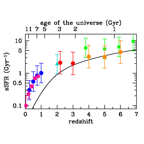 |
Figure 13. The mean specific star-formation rate (sSFR ≡ SFR / M∗) for galaxies with estimated stellar masses in the range 109.4-1010 M⊙. The values are from the literature: Daddi et al. (2007) (cyan triangle), Noeske et al. (2007) (blue dots), Damen et al. (2009) (magenta pentagons), Reddy et al. (2009) (red dots), Stark et al. (2013) (green squares), and González et al. (2014) (orange dots). The error bars correspond to systematic uncertainties. The high-redshift points from Stark et al. (2013) and González et al. (2014) have been corrected upward owing to the effect of optical emission lines on the derived stellar masses, using their "fixed Hα EW" model (Stark et al. 2013) and "RSF with emission lines" model (González et al. 2014). The curve shows the predictions from our best-fit star-formation history. |
According to Equation 4, the sum of the heavy elements stored in stars and in the gas phase at any given time, Zρg + < Z∗ > ρ∗, is equal to the total mass of metals produced over cosmic history, yρ∗. It can be useful to express this quantity relative to the baryon density,
 |
(18) |
where ρb = 2.77 × 10¹¹ Ωb h2 M⊙ Mpc-3. The evolution of the "mean metallicity of the Universe", Zb, predicted by our model SFH is plotted in Figure 14. The global metallicity is Zb≃ 0.09 (y / Z⊙) solar at the present epoch (note that this is the same value derived by Madau et al. 1998b). It drops to Zb≃ 0.01 (y / Z⊙) solar at z = 2.5, i.e., the star-formation activity we believe to have taken place between the Big Bang and z = 2.5 (2.5 Gyr later) was sufficient to enrich the Universe as a whole to a metallicity of ~ 1% solar (for y ≃ Z⊙). Note that the metal production term yρ∗ (and therefore Zb) depends only weakly on the IMF (at a fixed luminosity density): Salpeter-based mass-to-light ratios are 1.64 times higher than those based on Chabrier. This is counterbalanced by Salpeter-based net metal yields that are a factor of ~ 2 lower than those based on Chabrier (see Section 2).
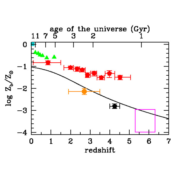 |
Figure 14. Mean metallicity of the Universe (in solar units): (solid curve) mass of heavy elements ever produced per cosmic baryon from our model SFH, for an assumed IMF-averaged yield of y = 0.02; (turquoise square) mass-weighted stellar metallicity in the nearby Universe from the SDSS (Gallazzi et al. 2008); (green triangles) mean iron abundances in the central regions of galaxy clusters (Balestra et al. 2007); (red pentagons) column density-weighted metallicities of the damped Lyα absorption systems (Rafelski et al. 2012); (orange dot) metallicity of the IGM as probed by O VI absorption in the Lyα forest (Aguirre et al. 2008); (black pentagon) metallicity of the IGM as probed by C IV absorption (Simcoe 2011); (magenta rectangle) metallicity of the IGM as probed by C IV and C II absorption (Ryan-Weber et al. 2009, Simcoe et al. 2011, Becker et al. 2011). |
Figure 14 also shows the metallicity of a variety of astrophysical objects at different epochs. The mass-weighted average stellar metallicity in the local Universe, < Z∗(0) > = (1.04 ± 0.14) Z⊙ (Gallazzi et al. 2008), is plotted together with the metallicity of three different gaseous components of the distant Universe: a) galaxy clusters, the largest bound objects for which chemical enrichment can be thoroughly studied, and perhaps the best example in nature of a "closed box"; b) the damped Lyα absorption systems that originate in galaxies and dominate the neutral-gas content of the Universe; and c) the highly ionized circumgalactic and intergalactic gas that participates in the cycle of baryons in and out of galaxies in the early Universe.
The iron mass in clusters is several times larger than could have been produced by CC SNe if stars formed with a standard IMF, a discrepancy that may indicate an IMF in clusters that is skewed toward high-mass stars (e.g., Portinari et al. 2004) and/or to enhanced iron production by Type Ia SNe (e.g., Maoz & Gal-Yam 2004). The damped Lyα absorption systems are detected in absorption (i.e., have no luminosity bias) and their large optical depths at the Lyman limit eliminates the need for uncertain ionization corrections to deduce metal abundances. Their metallicity is determined with the highest confidence from elements such as O, S, Si, Zn, and Fe and decreases with increasing redshift down to ≈ 1/600 solar to z ~ 5 (e.g., Rafelski et al. 2012). The enrichment of the circumgalactic medium, as probed in absorption by C III, C IV, Si III, Si IV, O VI, and other transitions, provides us with a record of past star formation and of the impact of galactic winds on their surroundings. Figure 14 shows that the ionization-corrected metal abundances from O VI absorption at z ~ 3 (Aguirre et al. 2008) and C IV absorption at z ~ 4 (Simcoe 2011) track well the predicted mean metallicity of the Universe, i.e. that these systems are an unbiased probe of the cosmic baryon cycle.
The Universe at redshift 6 remains one of the most challenging observational frontiers, as the high opacity of the Lyα forest inhibits detailed studies of hydrogen absorption along the line-of-sight to distant quasars. In this regime, the metal lines that fall longwards of the Lyα emission take on a special significance as the only tool at our disposal to recognize individual absorption systems, whether in galaxies or the IGM, and probe cosmic enrichment following the earliest episodes of star formation. Here, we used recent surveys of high- and low-ionization intergalactic absorption to estimate the metallicity of the Universe at these extreme redshifts. According to Simcoe et al. (2011) (see also Ryan-Weber et al. 2009), the comoving mass density of triply ionized carbon over the redshift range 5.3-6.4 is (expressed as a fraction of the critical density) ΩCIV = (0.46 ± 0.20) × 10-8. Over a similar redshift range, C II absorption yields ΩCII = 0.9 × 10⁻⁸ (Becker et al. 2011). The total carbon metallicity by mass, Zc, at < z> = 5.8 implied by these measurements is
 |
(19) |
where (C II + C IV) / C is the fraction of carbon that is either singly or triply ionized. In Figure 14, we plot Zc in units of the mass fraction of carbon in the Sun, ZC⊙ = 0.003 (Asplund et al. 2009). The lower bound to the rectangle centered at redshift 5.8 assumes no ionization correction, i.e., (C II + C IV)/C = 1. To derive the upper bound, we adopt the conservative limit (C II + C IV) / C ≥ 0.1; this is the minimum fractional abundance reached by C II + C IV under the most favorable photoionization balance conditions at redshift 6. [To obtain this estimate, we have computed photoionization models based on the CLOUDY code (Ferland et al. 1998) assuming the UV radiation background at z = 6 of Haardt & Madau (2012) and a range of gas overdensities 0 < logδ < 3.] If the ionization state of the early metal-bearing IGM is such that most of the C is either singly or triply ionized, then most of the heavy elements at these epochs appear to be "missing" compared with the expectations based on the integral of the cosmic SFH (Ryan-Weber et al. 2009, Pettini 2006). Conversely, if C II and C IV are only trace ion stages of carbon, then the majority of the heavy elements produced by stars 1 Gyr after the Big Bang (z = 6) may have been detected already.
A simple argument can also be made against the possibility that our best-fit SFH significantly overpredicts the cosmic metallicity at these early epoch. The massive stars that explode as Type II SNe and seed the IGM with metals are also the sources of nearly all of the Lyman-continuum (LyC) photons produced by a burst of star formation. It is then relatively straightforward to link a given IGM metallicity to the minimum number of LyC photons that must have been produced up until that time. The close correspondence between the sources of metals and photons makes the conversion from one to the other largely independent of the details of the stellar IMF (Madau & Shull 1996). Specifically, the energy emitted in hydrogen ionizing radiation per baryon, Eion, is related to the average cosmic metallicity by
 |
(20) |
where mp c2 = 938 MeV is the rest mass of the proton and η is the efficiency of conversion of the heavy element rest mass into LyC radiation. For stars with Z∗ = Z⊙ / 50, one derives η = 0.014 (Schaerer 2002, Venkatesan & Truran 2003). An average energy of 22 eV per LyC photon together with our prediction of Zb = 7 × 10⁻⁴ Z⊙ (assuming a solar yield) at redshift 6 imply that approximately 8 LyC photons per baryon were emitted by early galaxies prior to this epoch. Although at least one photon per baryon is needed for reionization to occur, this is a reasonable value because the effect of hydrogen recombinations in the IGM and within individual halos will likely boost the number of photons required. A global metallicity at z = 6 that was much lower than our predicted value would effectively create a deficit of UV radiation and leave the reionization of the IGM unexplained. In Section 5.8 below we link the production of LyC photons to stellar mass, show that the efficiency of LyC production decreases with increasing Z∗, and discuss early star formation and the epoch of reionization in more detail.
5.7. Black Hole Accretion History
Direct dynamical measurements show that most local massive galaxies host a quiescent massive black hole in their nuclei. Their masses correlate tightly with the stellar velocity dispersion of the host stellar bulge, as manifested in the MBH - σ∗ relation of spheroids (Ferrarese & Merritt 2000, Gebhardt et al. 2000). It is not yet understood whether such scaling relations were set in primordial structures and maintained throughout cosmic time with a small dispersion or which physical processes established such correlations in the first place. Nor it is understood whether the energy released during the luminous quasar phase has a global impact on the host, generating large-scale galactic outflows and quenching star formation (Di Matteo et al. 2005), or just modifies gas dynamics in the galactic nucleus (Debuhr et al. 2010).
Here, we consider a different perspective on the link between the assembly of the stellar component of galaxies and the growth of their central black holes. The cosmic mass accretion history of massive black holes can be inferred using Soltan's argument (Soltan 1982), which relates the quasar bolometric luminosity density to the rate at which mass accumulates into black holes,
 |
(21) |
where є is the efficiency of conversion of rest-mass energy into radiation. In practice, bolometric luminosities are typically derived from observations of the AGN emission at X-ray, optical or IR wavelengths, scaled by a bolometric correction. In Figure 15, several recent determinations of the massive black hole mass growth rate are compared with the SFRD (Equation 15). Also shown is the accretion history derived from the hard X-ray LF of Aird et al. (2010), assuming a radiative efficiency є = 0.1 and a constant bolometric correction of 40 for the observed 2-10 KeV X-ray luminosities. This accretion rate peaks at lower redshift than does the SFRD and declines more rapidly from z ≈ 1 to 0. However, several authors have discussed the need for luminosity-dependent bolometric corrections, which in turn can affect the derived accretion history (e.g., Marconi et al. 2004, Hopkins et al. 2007, Shankar et al. 2009). Moreover, although the hard X-ray LF includes unobscured as well as moderately obscured sources that may not be identified as AGN at optical wavelengths, it can miss Compton thick AGN, which may be identified in other ways, particularly using IR data. Delvecchio et al. (2014) have used deep Herschel and Spitzer survey data in GOODS-S and COSMOS to identify AGN by SED fitting. This is a potentially powerful method but depends on reliable decomposition of the IR emission from AGN and star formation.
Black hole mass growth rates derived from the bolometric AGN LFs of Shankar et al. (2009) and Delvecchio et al. (2014) are also shown in Figure 15. These more closely track the cosmic SFH, peaking at z ≈ 2, and suggest that star formation and black hole growth are closely linked at all redshifts (Boyle & Terlevich 1998, Silverman et al. 2008). However, the differences between accretion histories published in the recent literature would caution that it is premature to consider this comparison to be definitive.
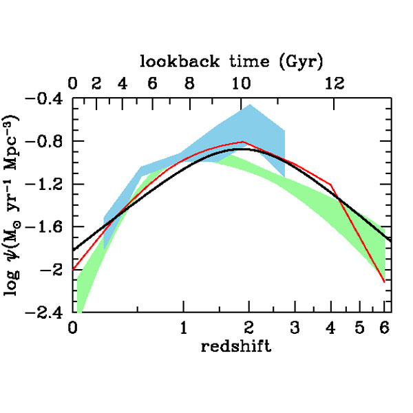 |
Figure 15. Comparison of the best-fit star formation history (thick solid curve) with the massive black hole accretion history from X-ray [red curve (Shankar et al. 2009); light green shading (Aird et al. 2010)] and infrared (light blue shading) (Delvecchio et al. 2014) data. The shading indicates the ± 1σ uncertainty range on the total bolometric luminosity density. The radiative efficiency has been set to є = 0.1. The comoving rates of black hole accretion have been scaled up by a factor of 3,300 to facilitate visual comparison to the star-formation history. |
5.8. First Light and Cosmic Reionization
Fundamental to our understanding of how the Universe evolved to its
present state is the epoch of "first light," the first billion years
after the Big Bang when the collapse of the earliest baryonic objects -
the elementary building blocks for the more massive systems that formed
later - determined the "initial conditions" of the cosmological
structure formation process. The reionization in the all-pervading IGM
- the transformation of neutral hydrogen into an ionized state - is a
landmark event in the history of the early Universe. Studies of Lyα
absorption in the spectra of distant quasars show that the IGM is highly
photoionized out to redshift z
6 (for a review, see
Fan et al. 2006),
whereas polarization data from the Wilkinson
Microwave Anisotropy Probe constrain the redshift of any sudden
reionization event to be significantly higher, z = 10.5 ± 1.2
(Jarosik et al. 2011).
It is generally thought that the IGM is kept
ionized by the integrated UV emission from AGN and star-forming
galaxies, but the relative contributions of these sources as a function
of epoch are poorly known (e.g.,
Madau et al. 1999,
Faucher-Giguère et
al. 2008,
Haardt & Madau 2012,
Robertson et al. 2013).
Establishing whether massive stars in young star-forming galaxies were responsible for cosmic reionization requires a determination of the early history of star formation, of the LyC flux emitted by a stellar population, and of the fraction of hydrogen-ionizing photons that can escape from the dense sites of star formation into the low-density IGM. We can use stellar population synthesis to estimate the comoving volumetric rate at which photons above 1 Ryd are emitted from star-forming galaxies as
 |
(22) |
where  ion is
expressed in units of
s-1 Mpc-3 and ψ in units of
M⊙ year-1 Mpc-3.
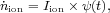
The LyC photon yield Iion is plotted in
Figure 16 for our reference Salpeter IMF and
for a wide range of metallicities spanning from extremely metal poor to
metal-rich stars
(Schaerer 2003).
The yield increases with decreasing metallicity by more than a factor of 3.
Integrating Equation 22 over time and dividing by the mean comoving
hydrogen density < nH > = 1.9 ×
10-7 cm-3, we can write the total number of
stellar LyC photons emitted per hydrogen atom since the Big Bang as
ion is
expressed in units of
s-1 Mpc-3 and ψ in units of
M⊙ year-1 Mpc-3.
The LyC photon yield Iion is plotted in
Figure 16 for our reference Salpeter IMF and
for a wide range of metallicities spanning from extremely metal poor to
metal-rich stars
(Schaerer 2003).
The yield increases with decreasing metallicity by more than a factor of 3.
Integrating Equation 22 over time and dividing by the mean comoving
hydrogen density < nH > = 1.9 ×
10-7 cm-3, we can write the total number of
stellar LyC photons emitted per hydrogen atom since the Big Bang as
 |
(23) |
where ρ∗(z) is the cosmic SMD. [Within
purely stellar radiation or energetic X-ray photons, either the total
number of ionizing photons produced or the total radiated energy,
respectively, is what matters for reionization. This is because, in a
largely neutral medium, each photoionization produces a host of
secondary collisional ionizations, with approximately one hydrogen
secondary ionization for every 37 eV of energy in the primary photoelectron
(Shull & van Steenberg
1985).
As the medium becomes more ionized, however, an increasing fraction of
this energy is deposited as heat.]
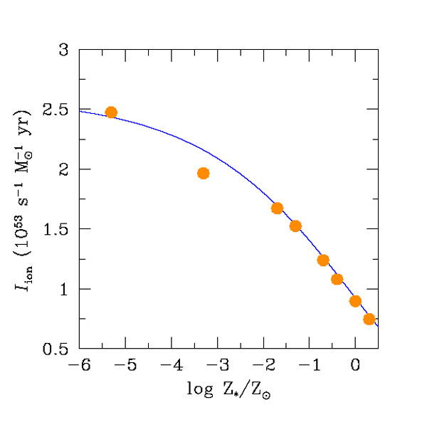
Figure 16 depicts the quantity
 ion at z
> 6 according to our best-fit SFH for the range of stellar
metallicities 0 < Z∗ <
Z⊙. Cosmological reionization requires at least
one LyC photon per hydrogen atom escaping into the intergalactic space,
i.e., ion
<fesc>; > 1. The exact number depends on the
rate of radiative recombinations in a clumpy IGM. Here, the escape
fraction < fesc> is the angle-averaged,
absorption cross-section-weighted, and luminosity-weighted fraction of
ionizing photons that leaks into the IGM from the dense star-forming
regions within galaxies.
ion at z
> 6 according to our best-fit SFH for the range of stellar
metallicities 0 < Z∗ <
Z⊙. Cosmological reionization requires at least
one LyC photon per hydrogen atom escaping into the intergalactic space,
i.e., ion
<fesc>; > 1. The exact number depends on the
rate of radiative recombinations in a clumpy IGM. Here, the escape
fraction < fesc> is the angle-averaged,
absorption cross-section-weighted, and luminosity-weighted fraction of
ionizing photons that leaks into the IGM from the dense star-forming
regions within galaxies.
 |
 |
Figure 16. (Left panel) Metallicity dependence of the ionizing photon yield, Iion, for a stellar population with a Salpeter IMF (initial mass function) and constant star-formation rate. The points show the values given in table 4 of Schaerer (2003), computed for a Salpeter IMF in the 1-100 M⊙ range, and divided by a mass conversion factor of 2.55 to rescale to a mass range 0.1-100 M⊙. The solid curve shows the best-fitting function, logIion = [(0.00038Z∗0.227 + 0.01858)]-1 - log(2.55). (Right panel) Number of H-ionizing photons emitted per hydrogen atom since the Big Bang, nion / < nH >, according to our best-fit star formation history. The shaded area is delimited by stellar populations with metallicities Z∗ = Z⊙ (lower boundary) and Z∗ = 0 (upper boundary). |
|
Figure 16 shows the well-known result that, even if the emission of LyC photons at early cosmic times was dominated by extremely low-metallicity stars, escape fractions in excess of 20% would be required to reionize the Universe by redshift 6-7 (e.g., Bolton & Haehnelt 2007, Ouchi et al. 2009, Bunker et al. 2010, Haardt & Madau 2012, Finkelstein et al. 2012b). Although the mechanisms regulating the escape fraction of ionizing radiation from galaxies and its dependence on cosmic time and luminosity are unknown, these leakage values are higher than typically inferred from observations of LBGs at z ~ 3 (e.g., Nestor et al. 2013, Vanzella et al. 2012, and references therein).
The "reionization budget" is made even tighter by two facts. First, the volume-averaged hydrogen recombination timescale in the IGM,
 |
(24) |
is ~ 60% of the expansion timescale H-1 = H0-1[ΩM(1 + z)3 + ΩΛ]-1/2 at z = 10, i.e., close to two ionizing photon per baryon are needed to keep the IGM ionized. Here, αb is the recombination coefficient to the excited states of hydrogen, χ = 1.08 accounts for the presence of photoelectrons from singly ionized helium, and CIGM is the clumping factor of ionized hydrogen. The above estimate assumes a gas temperature of 2 × 10⁴ K and a clumping factor for the IGM, CIGM = 1 + 43 z-1.71, that is equal to the clumpiness of gas below a threshold overdensity of 100 found at z ≥ 6 in a suite of cosmological hydrodynamical simulations (Pawlik et al. 2009; see also Shull et al. 2012). Second, the rest-frame UV continuum properties of very high redshift galaxies appear to show little evidence for the "exotic" stellar populations (e.g., extremely sub-solar metallicities or top-heavy IMFs) that would significantly boost the LyC photon yield (e.g., Finkelstein et al. 2012a, Dunlop et al. 2013). Although improved knowledge of the SFRD beyond redshift 9 may help to better characterize this photon shortfall, the prospects of a direct observational determination of the escape fraction of ionizing photons leaking into the IGM at these early epochs look rather bleak, as the Universe becomes opaque to LyC radiation above redshift 4.