Annu. Rev. Astron. Astrophys. 1999. 37:311-362 Copyright © 1999 by Annual Reviews. All rights reserved

2. PHYSICAL CONDITIONS

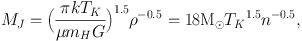
The motivation for studying physical conditions can be found in a few simple theoretical considerations. Our goal is to know when and how molecular gas collapses to form stars. In the simplest situation, a cloud with only thermal support, collapse should occur if the mass exceeds the Jeans (1928) mass,

(1)

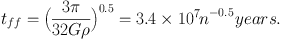
where T_K is the kinetic temperature (kelvins), ρ is the mass density (gm cm⁻³), and n is the total particle density (cm⁻³). In a molecular cloud, H nuclei are almost exclusively in H₂ molecules, and n ≃ n(H₂) + n(He). Then ρ = µ_n m_H n, where m_H is the mass of a hydrogen atom and µ_n is the mean mass per particle (2.29 in a fully molecular cloud with 25% by mass helium). Discrepancies between coefficients in the equations presented here and those in other references usually are traceable to a different definition of n. In the absence of pressure support, collapse will occur in a free-fall time (Spitzer 1978),

(2)

If T_K = 10 K and n ≥ 50 cm⁻³, typical conditions in the sterile regions (e.g. Blitz 1993), M_J ≤ 80 M_⊙, and t_ff ≤ 5 × 10⁶ years. Our Galaxy contains about 1–3 × 10⁹ M_⊙ of molecular gas (Bronfman et al 1988, Clemens et al 1988, Combes 1991). The majority of this gas is probably contained in clouds with M > 10⁴ M_⊙ (Elmegreen 1985). It would be highly unstable on these grounds, and free-fall collapse would lead to a star formation rate, ≥ 200 M_⊙yr⁻¹, far in excess of the recent Galactic average of 3 M_⊙yr⁻¹ (Scalo 1986). This argument, first made by Zuckerman & Palmer (1974), shows that most clouds cannot be collapsing at free fall (see also Zuckerman & Evans 1974). Together with evidence of cloud lifetimes of about 4 × 10⁷ yr (Bash et al 1977; Leisawitz et al 1989), this discrepancy motivates an examination of other support mechanisms.

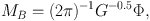
Two possibilities have been considered, magnetic fields and turbulence. Calculations of the stability of magnetized clouds (Mestel & Spitzer 1956, Mestel 1965) led to the concept of a magnetic critical mass (M_B). For highly flattened clouds,

(3)

(Li & Shu 1996), where Φ is the magnetic flux threading the cloud,

(4)

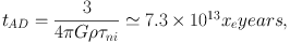
Numerical calculations (Mouschovias & Spitzer 1976) indicate a similar coefficient (0.13). If turbulence can be thought of as causing pressure, it may be able to stabilize clouds on large scales (e.g. Bonazzola et al 1987). It is not at all clear that turbulence can be treated so simply. In both cases, the cloud can only be metastable. Gas can move along field lines and ambipolar diffusion will allow neutral gas to move across field lines with a timescale of (McKee et al 1993)

(5)

where τ_ni is the ion-neutral collision time. The ionization fraction (x_e) depends on ionization by photons and cosmic rays, balanced by recombination. It thus depends on the abundances of other species (X(x) ≡ n(x) / n).

These two suggested mechanisms of cloud support (magnetic and turbulent) are not entirely compatible because turbulence should tangle the magnetic field (compare the reviews by Mouschovias 1999 and McKee 1999). A happy marriage between magnetic fields and turbulence was long hoped for; Arons and Max (1975) suggested that magnetic fields would slow the decay of turbulence if the turbulence was sub-Alfvénic. Simulations of MHD turbulence in systems with high degrees of symmetry supported this suggestion and indicated that the pressure from magnetic waves could stabilize clouds (Gammie & Ostriker 1996). However, more recent 3-D simulations indicate that MHD turbulence decays rapidly and that replenishment is still needed (Mac Low et al 1998, Stone et al 1999). The usual suggestion is that outflows generate turbulence, but Zweibel (1998) has suggested that an instability induced by ambipolar diffusion may convert magnetic energy into turbulence. Finally, the issue of supporting clouds assumes a certain stability and cloud integrity that may be misleading in a dynamic interstellar medium (e.g. Ballesteros-Paredes et al 1999). For a current review of this field, see Vázquez-Semadini et al (2000).

With this brief and simplistic review of the issues of cloud stability and evolution, we have motivated the study of the basic physical conditions:

(6)

All these are local variables; in principle, they can have different values at each point () in space and can vary with time (t). In practice, we usually can measure only one component of vector quantities, integrated through the cloud. For example, we measure only line-of-sight velocities, usually characterized by the linewidth (Δ v) or higher moments, and the line-of-sight magnetic field (B_z) through the Zeeman effect, or the projected direction (but not the strength) of the field in the plane of the sky (B_⊥) by polarization studies. In addition, our observations always average over finite regions, so we attempt to simplify the dependence on by assumptions or models of cloud structure. In Section 3, I will describe the methods used to probe these quantities and some overall results. Abundances have been reviewed recently (van Dishoeck & Blake 1998), so only relevant results will be mentioned, most notably the ionization fraction, x_e.

In addition to the local variables, quantities that explicitly integrate over one or more dimensions are often measured. Foremost is the column density,

(7)

The extinction or optical depth of dust at some wavelength is a common surrogate measure of N. If the column density is integrated over an area, one measure of the cloud mass within that area is obtained:

(8)

Another commonly used measure of mass is obtained by simplification of the virial theorem. If external pressure and magnetic fields are ignored,

(9)

where R is the radius of the region, Δ v is the FWHM linewidth, and the constant (C_v) depends on geometry and cloud structure, but is of order unity (e.g. McKee & Zweibel 1992, Bertoldi & McKee 1992). A third mass estimate can be obtained by integrating the density over the volume,

(10)

M_n is commonly used to estimate f_v, the volume filling factor of gas at density n, by dividing M_n by another mass estimate, typically M_v. Of the three methods of mass determination, the virial mass is the least sensitive to uncertainties in distance and size, but care must be taken to exclude unbound motions, such as outflows.

Parallel to the physical conditions in the gas, the dust can be characterized by a set of conditions:

(11)

where T_D is the dust temperature, n_D is the density of dust grains, and κ(ν) is the opacity at a given frequency, ν. If we look in more detail, grains have a range of sizes (Mathis et al 1977) and compositions. For smaller grains, T_D is a function of grain size. Thus, we would have to characterize the temperature distribution as a function of size, the composition of grains, both core and mantle, and many more optical constants to capture the full range of grain properties. For our purposes, T_D and κ(ν) are the most important properties, because T_D affects gas energetics and T_D and κ(ν) control the observed continuum emission of molecular clouds. The detailed nature of the dust grains may come into play in several situations, but the primary observational manifestation of the dust is its ability to absorb and emit radiation. For this review, a host of details can be ignored. The optical depth is set by

(12)

where it is convenient to define κ(ν) so that N is the gas column density rather than the dust column density. Away from resonances, the opacity is usually approximated by κ(ν) ∝ ν^β.