


The molecular ISM is typically cold and is observed at radio wavelengths. To search for the molecular ISM in galaxy outskirts one needs to be familiar with conventional notations in radio astronomy. Here we summarize the basic equations and assumptions that have been used in studies of the molecular ISM in traditional environments, such as in the MW's inner disk. In particular, we focus on the J = 1−0, 2−1 rotational transitions of CO molecules and dust continuum emission at millimetre/sub-millimetre wavelengths. The molecular ISM in galaxy outskirts may have different properties from those in the inner disks. We discuss how expected differences could affect the measurements with CO J = 1−0, 2−1, and dust continuum emission.
3.1. Brightness Temperature, Flux Density and Luminosity
The definitions of brightness temperature Tν, brightness Iν, flux density Sν, and luminosity Lν are often confusing. It is useful to go back to the amount of energy (dE) that passes through an aperture (e.g., detector, or sometimes the 4π sky area),
 |
(1) |
where Sν = ∫ Iν dΩB and Lν = ∫ ∫ Iν dΩB dA (see Fig. 1). The dt and dν denote unit time and frequency, respectively. The dΩB is the solid angle of the source and has the relation with the physical area dB = D2 dΩB with the distance D. Similarly, dA = D2 dΩA using the solid angle of the aperture area seen from the source dΩA. The aperture dA can be a portion of the 4π sky sphere as it is seen from the source and is 4π D2 when integrated over the entire sphere to calculate luminosity. The dA could also represent an area of a detector (or a pixel of a detector).
The flux density Sν is often expressed in the unit of “Jansky (Jy)”, which is equivalent to “10−23 erg s−1 cm−2 Hz−1”. An integration of Iν over a solid angle dΩB (e.g., telescope beam area or synthesized beam area) provides Sν. In reverse, Iν is Sν divided by the solid angle ΩB [= ∫ dΩB]. Therefore, the brightness Iν [= Sν / ΩB] is expressed in the unit of “Jy/beam”.
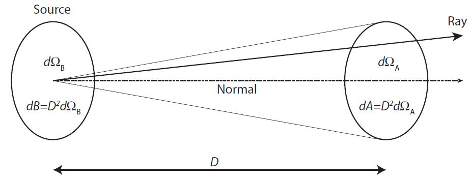 |
Figure 1. Definitions of parameters. The rays emitted from the source with the area dB = D2 dΩB pass through the solid angle dΩA (or the area D2 dΩA) at the distance of D |
The brightness temperature Tν is the temperature that makes the black body function Bν(Tν) have the same brightness as the observed Iν at a frequency ν (i.e., Iν = Bν(Tν)), even when Iν does not follow the black body law! In the Rayleigh-Jeans regime (hν ≪ kT),
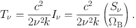 |
(2) |
The Tν characterizes radiation and is not necessarily a physical temperature of an emitting body. However, if the emitting body is an optically thick black body and is filling the beam ΩB, Tν is equivalent to the physical temperature of the emitting body when the Rayleigh-Jeans criterion is satisfied.
The Tν is measured in “Kelvin”. This unit is convenient in radio astronomy since radio single-dish observations calibrate a flux scale in the Kelvin unit using hot and cold loads of known temperatures. Giant molecular clouds (GMCs) in the MW have a typical temperature of ∼10 K (Scoville and Sanders (1987)), and the black body radiation Bν(T) at this temperature peaks at ν ∼ 588 GHz (∼ 510µm). Therefore, most radio observations of molecular gas are in the Rayleigh-Jeans range.
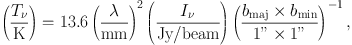
A numerical expression of Eq. (2) is useful in practice,
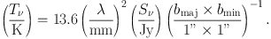 |
(3) |
The last term corresponds to ΩB in Eq. (2) and is calculated as
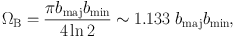 |
(4) |
which represents the area of interest (e.g., source size, telescope beam) as a 2-d Gaussian with the major and minor axis FWHM diameters of bmaj and bmin, respectively. Equation (3) is sometimes written with brightness as
 |
(5) |
where in this case the last term is for the unit conversion from “beam” into arcsec2, and bmaj and bmin must refer to the telescope beam or synthesized beam.
3.2. Observations of the Molecular ISM using CO Line Emission
Molecular hydrogen (H2) is the principal component of the ISM at a high density, > 100 cm−3. This molecule has virtually no emission at cold temperatures. Hence, CO emission is typically used to trace the molecular ISM. Conventionally, the molecular ISM mass Mmol includes the masses of helium and other elements. Mmol = 1.36 MH2 is used to convert the H2 mass into Mmol.
3.2.1. CO(J = 1−0) Line Emission
The fundamental CO rotational transition J = 1−0 at νCO(1−0) = 115.271208 GHz has been used to measure the molecular ISM mass since the 1980s. For simplicity we omit “CO(1−0)" in subscript and instead write “10". Hence, νCO(1-0) = ν10.
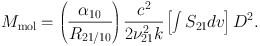
The dynamical masses of GMCs and their CO(1−0) luminosities are linearly correlated in the MW's inner disk (Scoville et al (1987); Solomon et al (1987)). If a great majority of molecules reside in GMCs, the CO(1−0) luminosity L10′ integrated over an area (i.e., an ensemble of GMCs in the area) can be linearly translated to the molecular mass Mmol,
 |
(6) |
where α10 (or XCO; see below) is a mass-to-light ratio and is called the CO-to-H2 conversion factor (Bolatto et al (2013)).
By convention we define L′10, instead of L10 (Eq. 1). With the CO(1−0) brightness temperature T10 (instead of Iν or I10), velocity width d v (instead of frequency width dν), and beam area in physical scale dB = D2 dΩB, it is defined as
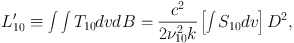 |
(7) |
where we used Eq. (2) for T10. The molecular mass is
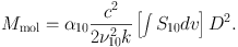 |
(8) |
Numerically, this can be expressed as
 |
(9) |
Note that S10 [= ∫ I10 dΩB] is an integration over an area of interest (or summation over all pixels within the area). The α10 = 4.3 M⊙ pc−2 corresponds to the conversion factor of XCO = 2.0 × 1020 cm−2 [K · km/s]−1 multiplied by the factor of 1.36 to account for the masses of helium and other elements. α10 includes helium, while XCO does not. The calibration of α10 (or XCO) is discussed in Bolatto et al (2013).
A typical GMC in the MW has a mass of 4 × 10⁵ M⊙ and dv = 8.9 km/s (FWHM) (Scoville and Sanders (1987)), which is ∫ S10 dv ∼ 1.5 Jy km/s or S10 ∼ 170 mJy at D = 5 Mpc.
3.2.2. CO(J = 2−1) Line Emission
The CO(J = 2−1) emission (230.538 GHz) is also useful for a rough estimation of molecular mass though an excitation condition may play a role (see below). We can redefine Eq. (8) for CO(2−1) by replacing the subscripts from 10 to 21 and using a new CO(2−1)-to-H2 conversion factor α21 ≡ α10 / R21/10, where R21/10 [≡ T21 / T10] is the CO J = 2−1/1−0 line ratio in brightness temperature.
In practice, α10 and R21/10 are carried over in use of CO(J = 2−1) as these are the parameters that have been measured. Equation (8) is now
 |
(10) |
A numerical evaluation gives
 |
(11) |
The typical GMC with 4 × 10⁵ M⊙ and dv = 8.9 km/s has ∫ S21 dv ∼ 4.2 Jy km/s or S21 ∼ 470 mJy at D = 5 Mpc. Note S21 > S10 for the same GMC because S21 / S10 = (ν21 / ν10)2 T21/ T10 = (ν21/ ν10)2 R21/10 ∼ 2.8 from Eq. (2), where the (ν21 / ν10)2 term arises from two facts: at the higher frequency, (a) each photon carries twice the energy, and (b) there are two times more photons in each frequency interval dν, which is in the denominator of the definition of flux density S. Empirically, R21/10 ∼ 0.7 on average in the MW (Sakamoto et al (1997); Hasegawa (1997)), which is consistent with a theoretical explanation under the conditions of the MW disk (Scoville and Solomon (1974); Goldreich and Kwan (1974); see Sect. 3.4).
3.3. Observations of the Molecular ISM using Dust Continuum Emission
Continuum emission from dust provides an alternative means for ISM mass measurement. Dust is mixed in the gas phase ISM, and its emission at millimetre/submillimetre waves correlates well with the fluxes of both atomic gas (Hi 21 cm emission) and molecular gas (CO emission). Scoville et al (2016) discussed the usage and calibration of dust emission for ISM mass measurement. We briefly summarize the basic equations, whose normalization will be adjusted with an empirical fitting in the end.
The radiative transfer equation gives the brightness of dust emission
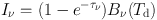 |
(12) |
with the black body radiation Bν(Td) at the dust temperature Td and the optical depth τν. The flux density of dust is an integration:
 |
(13) |
where Bν and τν are assumed constant within ΩB [= ∫ dΩB]. When the integration is over the beam area, Sν is the flux density within the beam, and (Sν / ΩB), from Eq. (13), is in Jy/beam.
An integration of Sν over the entire sky area at the distance of D (i.e., ∫ dA = D2 ∫ 4 π dΩA = 4 π D2) gives the luminosity
 |
(14) (15) |
The dust is optically thin at mm/sub-mm wavelengths, and we used (1 − e−τν) ∼ τν = κν Σd, where κν and Σd are the absorption coefficient and surface density of dust. The dust mass within the beam is Md = Σd D2 ΩB. Obviously, the dust continuum luminosity depends on the dust properties (e.g., compositions and size distribution; via κν), amount (Md), and temperature (Td).
Equation (15) gives the mass-to-light ratio for dust
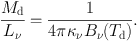 |
(16) |
We convert Md into gas mass, Mgas = δGDR Md, with the gas-to-dust ratio δGDR. By re-defining the dust absorption coefficient κ′ν ≡ κν / δGDR (the absorption coefficient per unit total mass of gas), the gas mass-to-dust continuum flux ratio γν at the frequency ν becomes,
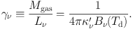 |
(17) |
Once γν is obtained, the gas mass is estimated as Mgas = γν Lν. Here, we use the character γ, instead of α that Scoville et al (2016) used, to avoid a confusion with the CO-to-H2 conversion factor. Dust continuum emission is associated with Hi and H2, and Mgas ∼ Mmol in dense, molecule-dominated regions (≳ 100 cm−3).
The κ′ν can be approximated as a power-law κ′ν = κ′850 µm (λ / 850 µm)−β with the spectral index β ∼ 1.8 (Planck Collaboration et al (2011)) and coefficient κ′850 µm at λ = 850 µm (352 GHz). In order to show the frequency dependence explicitly, we separate Bν(Td) into the Rayleigh-Jeans term and the correction term Γν(Td) as Bν(Td) = (2ν2k Td / c2) Γν(Td), where
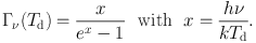 |
(18) |
Equation (17) has the dependence γν ∝ ν−(β + 2) Td−1 Γν(Td)−1, and the proportionality coefficient, including κ′850 µm and δGDR, is evaluated empirically.
Scoville et al (2016) cautioned that Td should not be derived from a spectral energy distribution fit (which gives a luminosity-weighted average Td biased toward hot dust with a peak in the infrared). Instead, they suggested to use a mass-weighted Td for the bulk dust component where the most mass resides. Scoville et al (2016) adopted Td = 25 K and calibrated γν850 µm from an empirical comparison of Mmol (from CO measurements) and Lν,
 |
(19) |
The luminosity is calculated from the observed Sν in Jy and distance D in centimetre as Lν = 4 π D2 Sν [Jy cm2]. The gas mass is then Mmol = γν Lν.
3.4. The ISM in Extreme Environments Such as the Outskirts
The methods for molecular ISM mass measurement that we discussed above were developed and calibrated mainly for the inner parts of galaxies. However, it is not guaranteed that these calibrations are valid in extreme environments such as galaxy outskirts. In fact, metallicities appear to be lower in the outskirts than in the inner part (see Bresolin, this volume). On a 1 kpc scale average, gas and stellar surface densities, and hence stellar radiation fields, are also lower, although it is not clear if these trends persist at smaller scales, e.g., cloud scales, where the molecular ISM typically exists. Empirically, α10 could be larger when metallicities are lower, and R21/10 could be smaller when gas density and/or temperature are lower.
In order to search for the molecular ISM and to understand star formation in the outskirts, it is important to take into account the properties and conditions of the ISM there. Here we explain some aspects that may bias measurements if the above equations are applied naively as they are. These potential biases should not discourage future research, and instead, should be adjusted continuously as we learn more about the ISM in the extreme environment.
3.4.1. Variations of α10 (or XCO)
The CO-to-H2 conversion factor α10 (or XCO) is a mass-to-light ratio between the CO(1−0) luminosity and the molecular ISM mass (Bolatto et al (2013)). Empirically, this factor increases with decreasing metallicity (Arimoto et al (1996); Leroy et al (2011)) due to the decreasing abundance of CO over H2. At the low metallicity of the small Magellanic cloud (∼ 1/10 Z⊙), α10 appears ∼ 10−20 times larger (Arimoto et al (1996); Leroy et al (2011)).
This trend can be understood based on the self-shielding nature of molecular clouds. Molecules on cloud surfaces are constantly photo-dissociated by stellar UV radiation. At high densities within clouds, the formation rate of molecules can be as fast as the dissociation rate, and hence molecules are maintained in molecular clouds. The depth where molecules are maintained depends on the strength of the ambient UV radiation field and its attenuation by line absorptions by the molecules themselves as well as by continuum absorption by dust (van Dishoeck and Black (1988)).
H2 is ∼ 104 times more abundant than CO. It can easily become optically thick on the skin of cloud surfaces and be self-shielded (Fig. 2). On the other hand, UV photons for CO dissociation penetrate deeper into the cloud due to its lower abundance.This process generates the CO-dark H2 layer around molecular clouds (Fig. 2b; Wolfire et al (2010)). Shielding by dust is more important for CO than H2. Therefore, if the metallicity or dust abundance is low, the UV photons for CO dissociation reach deeper and deeper, and eventually destroy all CO molecules while H2 still remains (Fig. 2c). As the CO-dark H2 layer becomes thicker, L10 decreases while MH2 stays high, resulting in a larger α10 in a low metallicity environment, such as galaxy outskirts. Since this process depends on the depth that photons can penetrate (through dust attenuation as well as line absorption), the visual extinction AV is often used as a parameter to characterize α10 (or XCO).
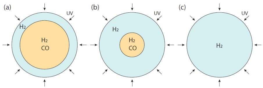 |
Figure 2. Self-shielding nature of molecules in molecular clouds. The abundance of molecules is maintained in clouds, since the destruction (photo-dissociation by UV radiation) and formation rates are in balance. The shielding from ambient UV radiation is mainly due to line absorption by molecules themselves. Therefore, the abundant H2 molecules become optically thick at the absorption line wavelengths on the skin of clouds, while UV photons for CO dissociation can get deeper into clouds. This mechanism generates the CO-dark H2 layer on the surface of molecular clouds. This layer can become thicker (panels a, b, c) under several conditions: e.g., lower metallicity or stronger local radiation field. The CO-to-H2 conversion factor α10 (or XCO) increases with the increasing thickness of the CO-dark H2 layer, and therefore, with lower metallicity or stronger local radiation field |
The CO(2−1) line emission is useful to locate the molecular ISM and to derive a rough estimation of its mass. However, the higher transitions inevitably suffer from excitation conditions. Indeed, R21/10 (≡ T21 / T10) has been observed to vary by a factor of 2−3 in the MW and in other nearby galaxies, e.g., between star-forming molecular clouds (typically R21/10 ∼ 0.7−1.0 and occasionally up to 1.2) and dormant clouds (∼ 0.4−0.7), and between spiral arms (> 0.7) and inter-arm regions (< 0.7; Sakamoto et al (1997); Koda et al (2012)). The variation may be negligible for finding molecular gas, but may cause a systematic bias, for example, in comparing galaxy outskirts with inner disks. It is noteworthy that R21/10 changes systematically with star formation activity, and varies along the direction of the Kennicutt-Schmidt relation, which can introduce a bias.
Theoretically, R21/10 is controlled by three parameters: the volume density nH2 and kinetic temperature Tk – which determine the CO excitation condition due to collisions – and the column density NCO, which controls radiative transfer and photon trapping (Scoville and Solomon (1974); Goldreich and Kwan (1974)). Figure 3 shows the variation of R21/10 with respect to nH2 and Tk under the large velocity gradient (LVG) approximation. In this approximation, the Doppler shift due to a cloud's internal velocity gradient is assumed to be large enough such that any two parcels along the line of sight do not overlap in velocity space. The front parcel does not block emission from the back parcel, and the optical depth is determined only locally within the parcel (or in small dv). Therefore, the column density is expressed per velocity NCO / dv. A typical velocity range in molecular clouds is adopted for this figure. An average GMC in the MW has nH2 ∼ 300 cm−3 and Tk ∼ 10 K (Scoville and Sanders (1987)), which results in R21/10 of ∼ 0.6−0.7. If the density and/or temperature is a factor of 2−3 higher due to a contraction before star formation or feedback from young stars, the ratio increases to R21/10 > 0.7. On the contrary, if a cloud is dormant compared to the average, the ratio is lower R21/10 < 0.7.
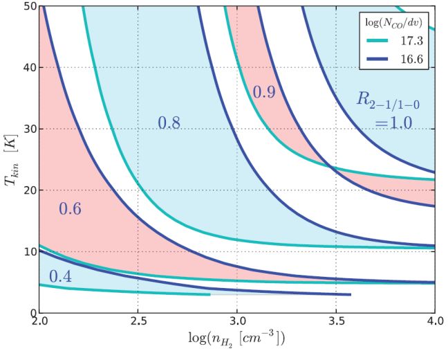 |
Figure 3. The CO J = 2−1 / 1−0 line ratios as function of the gas kinetic temperature Tkin and H2 density nH2 under the LVG approximation (from Koda et al (2012)). Most GMCs in the MW have CO column density in the range of log(NCO / dv) ∼ 16.6 to 17.3, assuming the CO fractional abundance to H2 of 8 × 10⁻⁵. An average GMC in the MW has nH2 ∼ 300 cm−3 and Tk ∼ 10 K, and therefore shows R21/10 ∼ 0.6-0.7. R21/10 is < 0.7 if the density and/or temperature decrease by a factor of 2−3, and R21/10 is >0.7 if the density and/or temperature increase by a factor of 2−3. Observationally, dormant clouds typically have R21/10 = 0.4−0.7, while actively star forming clouds have R21/10 = 0.7−1.0 (and occasionally up to ∼ 1.2; Sakamoto et al (1997); Hasegawa (1997)). There is also a systematic variation between spiral arms (R21/10 > 0.7) and interarm regions (R21/10 < 0.7; Koda et al (2012)) |
In the MW, cloud properties appear to change with the galactocentric radius (Heyer and Dame (2015)). If their densities or temperatures are lower in the outskirts, it would result in a lower R21/10, and hence, a higher H2 mass at a given CO(2−1) luminosity. If the R21/10 variation is not accounted for, it could result in a bias when clouds within the inner disk and in the outskirts are compared.
3.4.3. Variations of Dust Properties and Temperature
The gas mass-to-dust luminosity Mgas / Lν depends on the dust properties/emissivity (κν), dust temperature (Td), and gas-to-dust ratio (δGDR) – see Eqs. (16) and (17). All of these parameters could change in galaxy outskirts, which have low average metallicity, density, and stellar radiation field. Of course, the assumption of a single Td casts a limitation to the measurement as the ISM is multi-phase in reality, although the key idea of using Eqs. (16) and (17) is to target regions where the cold, molecular ISM is dominant (Scoville et al (2016)). The δGDR may increase with decreasing metallicity by about an order of magnitude (δGDR ∼ 40 → 400) for the change of metallicity 12 + log(O/H) from ∼ 9.0 → 8.0 (their Fig. 6; Leroy et al (2011)). If this trend applies to the outskirts, Eq. (17) would tend to underestimate the gas mass by up to an order of magnitude.
Excess dust emission at millimetre/submillimetre wavelengths has been reported in the small and large Magellanic clouds (SMC and LMC) and other dwarfs (Bot et al (2010); Dale et al (2012); although see also Kirkpatrick et al (2013)). This excess emission appears significant when spectral energy distribution fits to infrared data are extrapolated to millimetre/submillimetre wavelengths. Among the possible explanations are the presence of very cold dust, a change of the dust spectral index, and spinning dust emission (e.g., Bot et al (2010)). Gordon et al (2014) suggested that variations in the dust emissivity are the most probable cause in the LMC and SMC from their analysis of infrared data from the Herschel Space Observatory. The environment of galaxy outskirts may be similar to those of the LMC/SMC. The excess emission (27% and 43% for the LMC and SMC, respectively; Gordon et al (2014)) can be ignored if one only needs to locate dust in the vast outskirts, but could cause a systematic bias when the ISM is compared between inner disks and outskirts.