Copyright © 2015 by Annual Reviews. All rights reserved
| Annu. Rev. Astron. Astrophys. 2015. 53:115-154
Copyright © 2015 by Annual Reviews. All rights reserved |


We have seen from Section 2 that a large
fraction of observed AGN show ultrafast outflows. Unless we view every
AGN from a very particular angle (so implying a much larger total
population) this must mean that these winds have large solid angles
4π b with b ∼ 1, i.e. they are
quasispherical. We recall that UFOs are observed to have total scalar
momenta ∼ LEdd / c, where
LEdd is the Eddington luminosity of the SMBH. We can
argue that on quite general grounds, SMBH mass growth is likely to occur
at accretion rates close to the value
 Edd =
LEdd / η c2 which would
produce this luminosity. As we noted earlier, the
Soltan (1982)
relation shows that the largest SMBH gained most of their mass by luminous
accretion, i.e. during AGN phases. But the fraction of AGN among all
galaxies is small, strongly suggesting that when SMBH grow, they
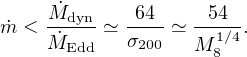
are likely to do so as fast as possible. The maximum possible rate of
accretion from a galaxy bulge with velocity dispersion σ
is the dynamical value
Edd =
LEdd / η c2 which would
produce this luminosity. As we noted earlier, the
Soltan (1982)
relation shows that the largest SMBH gained most of their mass by luminous
accretion, i.e. during AGN phases. But the fraction of AGN among all
galaxies is small, strongly suggesting that when SMBH grow, they
are likely to do so as fast as possible. The maximum possible rate of
accretion from a galaxy bulge with velocity dispersion σ
is the dynamical value
 |
(15) |
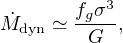
where fg is the gas fraction. This rate applies when
gas which was previously in gravitational equilibrium is disturbed and
falls freely, since one can estimate that the gas mass
was roughly Mg ∼ σ2
fg R / G. Once this is destabilized it
must fall inwards on a dynamical timescale tdyn
∼ R/σ. This gives the result (15), since
dyn
∼ Mg / tdyn.
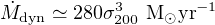
Numerically we have
 |
(16) |
where we have taken fg = 0.16, the cosmological baryon fraction of all matter. We have
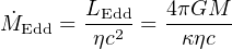 |
(17) |
where LEdd is the Eddington luminosity and κ is the electron scattering opacity. With η = 0.1 and black hole masses M close to the observed M − σ relation (2) we find
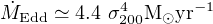 |
(18) |
and an Eddington accretion ratio
 |
(19) |
Thus even dynamical infall cannot produce extremely super–Eddington accretion rates on to supermassive black holes. But the rate (15) is already a generous overestimate, since it assumes that the infalling gas instantly loses all its angular momentum. Keeping even a tiny fraction of this instead forces the gas to orbit the black hole and form an accretion disc, which slows things down drastically. Gas spirals inwards through a disc on the viscous timescale
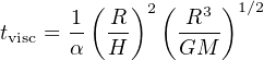 |
(20) |
where α ∼ 0.1 is the Shakura–Sunyaev viscosity parameter, while the disc aspect ratio H / R is almost constant with radius, and typically close to 10−3 for an AGN accretion disc (e.g. Collin-Souffrin & Dumont 1990). Then tvisc approaches a Hubble time even for disc radii of only 1 pc. Gas must evidently be rather accurately channelled towards the SMBH in order to accrete at all, constituting a major problem for theories of how AGN are fuelled.
Given all this, we see that while it is possible for AGN accretion rates
to reach Eddington ratios  ∼ 1, significantly larger ones are unlikely unless the SMBH mass
is far below the M − σ value appropriate to the
galaxy bulge it inhabits. In other words, only relatively modest values
∼ 1 of the
Eddington ratio are likely in SMBH growth episodes.
∼ 1, significantly larger ones are unlikely unless the SMBH mass
is far below the M − σ value appropriate to the
galaxy bulge it inhabits. In other words, only relatively modest values
∼ 1 of the
Eddington ratio are likely in SMBH growth episodes.
Indirect evidence supporting this view comes from stellar–mass
compact binary systems. The dynamical rate is relatively much larger
here, as the equivalent of (15) is
∼
vorb3 / G ∼
M2 / P, with vorb the orbital
velocity of a companion star in a binary of period P. This
implies rates approaching a solar mass per few hours in many cases, if
dynamical accretion ever occurs. These systems have highly
super–Eddington apparent luminosities, probably as the result of
geometric collimation (cf
King et al. 2001).
But significantly there are no obvious AGN analogues of the
ultra-luminous X-ray sources (ULXs), suggesting that Eddington ratios
≫ 1 are very
unusual or absent in AGN.
Given this, we can crudely model the UFOs discussed in
Section 2 as
quasi-spherical winds from SMBH accreting at modest Eddington ratios
=
/
Edd
∼ 1. Winds like this have electron
scattering optical depth τ ∼ 1, measured inwards from
infinity to a distance of order the Schwarzschild radius
(cf eq. 27 below). So on average every
photon emitted by the AGN scatters about once before escaping to
infinity. Since electron scattering is front–back symmetric, each
photon on average gives up all its momentum to the wind, and so the
total (scalar) wind momentum should be of order the photon momentum, or
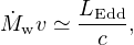 |
(21) |
where v is the wind's terminal velocity. The winds of hot stars obey relations like this. For accretion from a disc, as here, the classic paper of Shakura & Sunyaev (1973) finds a similar result at super–Eddington mass inflow rates: the excess accretion is expelled from the disc in a quasispherical wind.
Equation (17) now directly gives the wind terminal velocity as
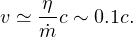 |
(22) |
From eq. (22) we get the instantaneous wind mechanical luminosity as
 |
(23) |
This relation turns out to be highly significant (see Sections 5.3, 7.3).
Ohsuga & Mineshige (2011) show in detail that winds with these properties (their Models A and B) are a natural outcome of mildly super–Eddington accretion. In particular their Model A and B winds are predicted (cf their Figure 3) to have mechanical luminosities ∼ 0.1LEdd, in rough agreement with equation (23).
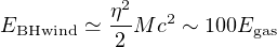
Compared with the original disparity EBH = η Mc2 ∼ 2000 Egas between black hole and bulge gas binding energies outlined in the Introduction, we now have a relation
 |
(24) |
between the available black hole wind mechanical energy and the bulge binding energy. Although the mismatch is less severe, it still strongly suggests that the bulge gas would be massively disrupted if it experienced the full mechanical luminosity emitted by the black hole for a significant time. So the coupling of mechanical energy to the host ISM cannot be efficient all the time (see the discussion in Section 2). We show how this works in Section 4.
As we have seen, observations frequently give the hydrogen column density NH through a UFO wind from the X–ray absorption spectrum. We can show that this quantity determines whether a given UFO wind is observable or not. Using (21) in the mass conservation equation
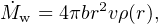 |
(25) |
where ρ(r) is the mass density, we find the equivalent hydrogen column density of the wind as
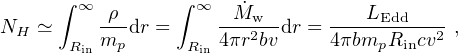 |
(26) |
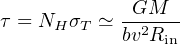
where Rin is its inner radius, mp is the proton mass, and we have used (21) at the last step. From the definition of LEdd we find the wind electron scattering optical depth
 |
(27) |
with σT ≃ κ mp the Thomson cross–section. This shows self–consistently that the scattering optical depth τ of a continuous wind is ∼ 1 (cf King & Pounds 2003, equation 4) at the launch radius Rlaunch ≃ GM / bv2 = (c2 / 2bv2) Rs ≃ 50Rs.
The measured values of NH (Tombesi et al. 2011, Gofford et al. 2013, Figure 4) are always smaller than the value NH ≃ 1/σT ≃ 1024 cm−2 for a continuous wind, and actually lie in the range N22 ∼ 0.3 − 30, where N22 = NH / 1022 cm−2. It is perhaps not surprising that observations do not show any UFO systems with NH > 1024 cm−2. These AGN would be obscured at all photon energies by electron scattering, and perhaps difficult to see. Although such systems might be common, we probably cannot detect them. To have a good chance of seeing a UFO system we need a smaller NH, so from (27) the inner surface Rin of the wind must be larger than Rlaunch. This is only possible if all observed UFOs are episodic, i.e. we see them some time after the wind from the SMBH has switched off. In this sense UFOs are more like a series of sporadically–launched quasispherical shells than a continuous outflow. The NH value of each shell is dominated by the gas near its inner edge (cf (26), so we probably at most detect only the inner edge of the most recently–launched shell. We can quantify this by setting Rin = vtoff, where toff is the time since the launching of the most recent wind episode ended. Using (27) gives
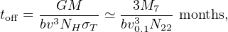 |
(28) |
where v0.1 = v / 0.1c.
As seen in Figure 4, all UFOs have N22 ∼ 0.3 − 30, and most of the SMBH masses are ∼ 107 M⊙. Evidently the launches of most observed UFO winds halted weeks or months before the observation. At first sight this is surprising. The strength of the characteristic blueshifted absorption features defining UFOs is closely related to NH. These features would be still stronger if there were UFOs with N22 > 100, but none are seen. We note from (28) that observing a UFO like this would require us to catch it within days of launch. Given the relatively sparse coverage of X–ray observations of AGN this is unlikely. So the apparent upper limit to the observed NH may simply reflect a lack of observational coverage, and implies that most UFOs are short-lived.
The lower limit to NH in the Tombesi et al. sample is also interesting. Once NH is smaller than some critical value, any blueshifted absorption lines must become too weak to detect. The strongest are the resonance lines of hydrogen– and helium–like iron, which have absorption cross–sections σFe ≃ 10−18 cm2. Given the abundance by number of iron as ZFe = 4 × 10⁻⁵ times that of hydrogen, the condition that one of these lines should have significant optical depth translates to ZFe NH σFe > 1 or N22 > 2.5. This is similar to the lowest observed values. From (28) this means that current observations cannot detect UFO winds launched more than a few months in the past, because the blueshifted iron lines will be too weak. Even these observed UFOs should gradually decrease their NH and become unobservable if followed for a few years. We see in Section 5 that the UFO wind typically travels ∼ 10M7 pc or more before colliding with the host galaxy’s interstellar gas, which takes tcoll / v ∼ 300M7 v0.1−1 yr. Finally, a UFO may be unobservable simply because it is too strongly ionized, so that no significant NH can be detected.
All this means that the state of the AGN seen in a UFO detection does not necessarily give a good idea of the conditions required to launch it. In particular, the AGN may be observed at a sub–Eddington luminosity, even though one might expect luminosities ∼ LEdd to be needed for launching the UFO. This may be the reason why AGN showing other signs of super–Eddington phenomena (e.g. narrow–line Seyfert 2 galaxies) are nevertheless seen to have sub–Eddington luminosities most of the time (e.g. NGC 4051; Denney et al. 2009): the rather short wind episodes are launched in very brief phases in which accretion is slightly super–Eddington, whereas the long–term average rate of mass gain may be significantly sub–Eddington.
In summary, it is likely that current UFO coverage is remarkably sparse. We cannot see a continuous wind at all. We can only see an episodic wind shell shortly after launch, and then only for a tiny fraction toff / tcoll ∼ 10−3 v0.1−2 N22−1 of its ∼ 300 − 3000 yr journey to collision with the host ISM. So it seems that the vast majority of UFO wind episodes remain undetected: more AGN must produce them than we observe, and the known UFO sources may have far more episodes than we detect.
All this has important consequences for how we interpret observations in discussing feedback. The most serious is that the most powerful form of feedback – from AGN at the Eddington limit producing continuous winds – is probably not directly observable at all.
3.4. The Wind Ionization State, and BAL QSOs
 |
(29) |
essentially fixes the ionization state of a black hole wind wind, and so determines which spectral lines are observed. Here Li = li LEdd is the ionizing luminosity, with li < 1 a dimensionless parameter specified by the quasar spectrum, and N = ρ / µmp is the number density of the UFO gas. We use (22, 25) to get
 |
(30) |
where l2 = li / 10−2, and η0.1 = η / 0.1.
This relation shows how the wind momentum and mass rates determine its ionization parameter and so its line spectrum as well as its speed v. Given a quasar spectrum Lν , the ionization state has to arrange that the threshold photon energy defining Li, and the corresponding ionization parameter ξ, together satisfy (30). This shows that the excitation must be high: a low threshold photon energy (say in the infrared) would imply a large value of l2, but then (30) gives a high value of ξ and so predicts the presence of very highly ionized species, physically incompatible with such low excitation.
For suitably chosen continuum spectra (30) has a range of solutions. A
given spectrum might in principle allow more than one solution, the
applicable one being specified by initial conditions. For a
typical quasar spectrum, an obvious self–consistent solution of
(30) is l2 ≃ 1,
≃ 1, ξ
≃ 3 × 10⁴. Here the quasar radiates the
Eddington luminosity. We can also consider situations where the quasar's
luminosity has decreased after an Eddington episode but the wind is
still flowing, with
≃ 1. Then the ionizing luminosity 10−2
l2 LEdd in
(30) is smaller, implying a lower ξ. As an example, an AGN of
luminosity 0.3LEdd would have ξ ∼
104. This gives a photon energy threshold appropriate to
FeXXV and Fe XXVI (i.e. hνthreshold ∼ 9
keV). We conclude that Eddington winds from AGN are likely to have
velocities ∼ 0.1c, and show the presence of helium–
or hydrogen-like iron in accord with the absorption reported in
Section 2.
Zubovas & King (2013)
show that this probably holds even for AGN which are significantly
sub–Eddington.
We can see from (22) that a larger Eddington factor
is likely to
produce a slower wind. From comparison with ULXs (see
Section 3.1) we also expect the AGN radiation to be
beamed away from a large fraction of the UFO, which should therefore be
be less ionized, and as a result more easily detectable than the small
fraction receiving the beamed radiation. These properties –
slower, less ionized winds – characterize BAL QSO outflows,
perhaps suggesting that systems with larger
> 1 appear as BAL
QSOs.
Zubovas & King (2013)
tentatively confirm this idea.