


Now consider what we know empirically about the abundance of radio AGN at high redshift, and what constraints this information may set on models of structure formation.
No significant new datasets relevant to the luminosity function of powerful radio sources have been published since the study of the RLF published by James Dunlop and myself in 1990. This was based on nearly-complete redshift data on roughly 500 sources down to a limit of 100 mJy at 2.7 GHz, plus fainter number-count data and partial identification statistics.
The main conclusions of this study were firstly to affirm long-standing
results
(Longair 1966;
Wall, Pearson &
Longair 1980)
that the RLF undergoes differential evolution:
the highest luminosity sources change their comoving densities
fastest. Nevertheless,
because the RLF curves, the results can be described by a model of pure
luminosity
evolution for the high-power population, in close analogy with the
situation for optically-selected quasars
(Boyle et al. 1988).
The characteristic luminosity in this case
increases by a factor  20
between the present and a redshift of 2. Similar behavior applies
for both steep-spectrum and fiat-spectrum sources, which provides some
comfort for those
wedded to unified models for the AGN population. There is a remarkable
similarity here
to the evolution of `starburst' galaxies, distinguished by blue
optical-UV continua and
strong emission from dust which make them very bright in the IRAS
60-µm band. It has been increasingly clear since the work of
Windhorst (1984)
that such galaxies make
up a substantial part of the radio-source population below S
1 mJy. The evolution of
these objects at radio wavelengths and at 60 µm is directly related
because there exists
an excellent correlation between output at these two wavebands.
Rowan-Robinson et
al. (1993)
have exploited this to investigate the implications of IRAS evolution
for the faint
radio counts. They find good consistency with the luminosity evolution
L
20
between the present and a redshift of 2. Similar behavior applies
for both steep-spectrum and fiat-spectrum sources, which provides some
comfort for those
wedded to unified models for the AGN population. There is a remarkable
similarity here
to the evolution of `starburst' galaxies, distinguished by blue
optical-UV continua and
strong emission from dust which make them very bright in the IRAS
60-µm band. It has been increasingly clear since the work of
Windhorst (1984)
that such galaxies make
up a substantial part of the radio-source population below S
1 mJy. The evolution of
these objects at radio wavelengths and at 60 µm is directly related
because there exists
an excellent correlation between output at these two wavebands.
Rowan-Robinson et
al. (1993)
have exploited this to investigate the implications of IRAS evolution
for the faint
radio counts. They find good consistency with the luminosity evolution
L  (1 +
z)3
reported for the complete `QDOT' sample of IRAS galaxies by
Saunders et
al. (1990).
(1 +
z)3
reported for the complete `QDOT' sample of IRAS galaxies by
Saunders et
al. (1990).
Were it not for the fact that some populations of objects show little evolution (e.g. normal galaxies in the near-infrared: Glazebrook 1991), one might be tempted to suggest an incorrect cosmological model as the source of this near-universal behavior. The alternative is to look for an explanation which owes more to global changes in the Universe than in the detailed functioning of AGN. One obvious candidate, long suspected of playing a role in AGN, is galaxy mergers; Carlberg (1990) suggested that this mechanism could provide evolution at about the right rate (although see Lacey & Cole 1993). Why the evolution does not look like density evolution is still a major stumbling block, but it seems that we should be looking at this area quite intensively, given that mergers have been implicated in both AGN and starbursts, and that there may be some evidence for their operation from the general galaxy population (Broadhurst, Ellis & Glazebrook 1992).
However, it is unclear how much emphasis should be placed on this apparent
universality; particularly, limited statistics make it uncertain just
how well luminosity evolution is obeyed. For example,
Goldschmidt et
al. (1992)
have produced evidence
that the PG survey is very seriously incomplete at z
 1; if confirmed, this
would imply
that the evolution of quasars of the very highest luminosities is less
than for those a
few magnitudes weaker. Furthermore, the QDOT database was afflicted by
an error in
which 10% of the galaxies were assigned incorrectly high redshifts
(Lawrence, private
communication); this will probably weaken the IRAS degree of
evolution. It may well
be that the degree of unanimity described above will prove spurious, and
that we will
be left with the unsurprising situation that a complex phenomenon like
AGN evolution
can only be described simply when the samples are too small to show much of the
detail.
1; if confirmed, this
would imply
that the evolution of quasars of the very highest luminosities is less
than for those a
few magnitudes weaker. Furthermore, the QDOT database was afflicted by
an error in
which 10% of the galaxies were assigned incorrectly high redshifts
(Lawrence, private
communication); this will probably weaken the IRAS degree of
evolution. It may well
be that the degree of unanimity described above will prove spurious, and
that we will
be left with the unsurprising situation that a complex phenomenon like
AGN evolution
can only be described simply when the samples are too small to show much of the
detail.
4.2 Redshift cutoff and interpretation
At higher redshifts, the uncertainties increase as the data thin out,
but there is
evidence that the luminosity function cannot stay at its z = 2
value at all higher
redshifts. The form of this `redshift cutoff' is uncertain: we cannot at
present distinguish
between possibilities such as a gradual decline for z > 2, or a
constant RLF up to some
critical redshift, followed by a more precipitous decline. We therefore
present a `straw
man' model designed to concentrate the minds of observers, in which the
luminosity
evolution goes into reverse at z
2 and the characteristic
luminosity retreats by a
factor 3 by z = 4
(Figure 2).

|
Figure 2. The evolving RLF, according to
the pure luminosity evolution model of
Dunlop & Peacock
(1990).
The main features are a break which moves to higher powers
at high redshift, but which declines slightly at z
|
This model predicts the following fraction of objects at z > 3.5
as a function of
1.4-GHz flux-density limit: 0.5% at 100 mJy; 3% at 1 mJy. Without some form of
cutoff, these numbers would be about a factor of 5 higher. The reason
for the increased
ease of detecting a cutoff at low flux density is that the RLF is rather
flat at low
powers; for  P-
P- and S
and S
 -
- , we expect dN / dz
(1 + z)-(2+)-1/2. Steep
spectra and a steep RLF thus discriminate against high redshifts, but at
low powers
the flatter RLF helps us to see whatever high-z objects there are
more easily. It should
be relatively easy to test for the presence of a cutoff on the basis of
these predictions. This is especially true at low flux densities (see
Figure 3). Here, we still sample the flat
portion of the RLF even at high redshift, and so the predicted numbers
of high-redshift
sources is large without a cutoff - around 15% at z > 4 for a
sample at 1 mJy.
, we expect dN / dz
(1 + z)-(2+)-1/2. Steep
spectra and a steep RLF thus discriminate against high redshifts, but at
low powers
the flatter RLF helps us to see whatever high-z objects there are
more easily. It should
be relatively easy to test for the presence of a cutoff on the basis of
these predictions. This is especially true at low flux densities (see
Figure 3). Here, we still sample the flat
portion of the RLF even at high redshift, and so the predicted numbers
of high-redshift
sources is large without a cutoff - around 15% at z > 4 for a
sample at 1 mJy.

|
Figure 3. A plot of the integral redshift
distributions predicted for two samples limited
at 1.4-GHz flux densities of 100 mJy and 1 mJy. The upper line shows a
prediction
for a luminosity function which is held constant for z
|
Whether or not the redshift cutoff is real, we seem to have direct
evidence that the
characteristic comoving density of radio galaxies has not altered
greatly between z 4
and the present. Integrating to 1 power of 10 below the break in the
RLF, we find
|
Is this a surprising number? In models involving hierarchical collapse, the characteristic mass of bound objects is an increasing function of time. At high mass, the abundance of objects falls exponentially if the statistics of the density field are Gaussian. Clearly, a model such as CDM (which falls in this class) will be embarrassed if the density of massive objects stays high to indefinite redshifts. The analysis of this problem, using the Press-Schechter mass-function formalism (Press & Schechter 1974) was first given by Efstathiou & Rees (1988) for optically-selected quasars.
There are two degrees of freedom in the analysis: what mass of object is under
study, and what are the parameters of the fluctuation power spectrum?
For the first,
Efstathiou & Rees had to construct a long and uncertain chain of
inference leading from
quasar energy output, to black-hole mass, to baryonic galaxy mass, to
total halo mass.
For radio galaxies, things are much simpler, because we can see the
galaxy directly.
Infrared observations imply that, certainly up to z = 2, the
stellar mass of radio galaxies
has not changed significantly. At low redshift, there is direct evidence
that the mass of radio galaxies exceeds 1012
M , so it seems
reasonable to adopt this value at higher
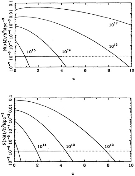
redshift. Figure 4 shows the Press-Schechter
predictions for two COBE-normalized
CDM models. The low-h model which fits the shape of the
galaxy-clustering power spectrum
(Peacock 1991)
intersects the observed number density at low-ish redshifts
(7-8), whereas the `standard' h = 0.5 model with its higher
degree of small-scale power
predicts many more objects. This is clearly only a suggestive
coincidence at present, but
it is clearly interesting that the model which most nearly describes
large-scale structure
also predicts that the formation of massive objects should occur near
the point at which we infer a lack of high-z AGN.
, so it seems
reasonable to adopt this value at higher
redshift. Figure 4 shows the Press-Schechter
predictions for two COBE-normalized
CDM models. The low-h model which fits the shape of the
galaxy-clustering power spectrum
(Peacock 1991)
intersects the observed number density at low-ish redshifts
(7-8), whereas the `standard' h = 0.5 model with its higher
degree of small-scale power
predicts many more objects. This is clearly only a suggestive
coincidence at present, but
it is clearly interesting that the model which most nearly describes
large-scale structure
also predicts that the formation of massive objects should occur near
the point at which we infer a lack of high-z AGN.
|
Figure 4. The epoch dependence of the
integral mass function in CDM, calculated
using the Press-Schechter formalism as in
Efstathiou & Rees
(1988).
The normalization
is to the COBE detection of CMB fluctuations. Results are shown for two Hubble
constants: the `standard'
|
In the spirit of this meeting, it is probably important to concentrate on integrated properties of the radio-source population. One important feature of this sort is the relic density of black holes deposited by the work of past AGN. This is something which has been discussed extensively for radio-quiet quasars, but which has not been given so much attention in the radio waveband alone. The advantage of doing this is that, as discussed above, we have a rather good idea of which galaxies host radio-loud AGN, and therefore we know where to look for any debris from burned-out AGN. The basic analysis of this problem goes back to Soltan (1982). He showed that the relic black-hole density may be deduced observationally in a model-independent manner, as follows.
The mass deposited into black holes in time dt by an AGN of
luminosity L is
|
where  is an efficiency,
and g is a bolometric correction. To obtain the total mass
density in black holes, we have to multiply the above equation by the
luminosity function
(which already gives the comoving density, as required) and integrate
over luminosity.
The integral can be converted to one over redshift and flux density, and
the integrand
depends of the observable distribution of redshifts and flux densities,
so the answer is
model dependent. Doing this for the Radio LF gives a much lower answer than for
optically-selected QSOs, which have a much higher density:
is an efficiency,
and g is a bolometric correction. To obtain the total mass
density in black holes, we have to multiply the above equation by the
luminosity function
(which already gives the comoving density, as required) and integrate
over luminosity.
The integral can be converted to one over redshift and flux density, and
the integrand
depends of the observable distribution of redshifts and flux densities,
so the answer is
model dependent. Doing this for the Radio LF gives a much lower answer than for
optically-selected QSOs, which have a much higher density:
|
Since we know rather well the present density of massive elliptical galaxies (e.g. Loveday et al. 1992), we may distribute half the above radio mass into ellipticals above the median radio-galaxy luminosity, with the following result for the mean hole mass:
|
What is the bolometric correction for radio galaxies? We know that the total output generally peaks in the IRAS wavelength regime, with an effective g ~ 100 (Heckman, Chambers & Postman 1992); this gives
|
which paints a rather less optimistic prospect for detection than
studies based on the
output of QSOs. This is because, even with such a large g, the
actual energy radiated
by radio galaxies is rather low, and this is not compensated for fully
by the relative
rareness of the host galaxies. The above figure is not easy to reconcile
with large
black-hole masses suggested for some radio AGN. For example,
Lauer et al. (1992)
suggest a central mass of
M 3 x 10⁹
M for
M87. Without suggesting that M87 is
greatly atypical, this can always be made consistent by assuming a low
enough efficiency.
However, this would not fit well with the view that radio galaxies are
powered via
electrodynamic extraction of black-hole rotational energy (e.g.
Blandford 1990);
here the efficiency can be up to
= 1 - 2-1/2. If
masses of order 109
M are substantiated
in several radio galaxies or radio-quiet massive ellipticals, this would
be quite a puzzle.
Probably the simplest solution would be to suggest that the total energy
was higher
than suggested by the above sum - perhaps because radio ellipticals
spend part of their
lives as QSOs, where the total energy output would be considerably
higher for a given radio power.
3 x 10⁹
M for
M87. Without suggesting that M87 is
greatly atypical, this can always be made consistent by assuming a low
enough efficiency.
However, this would not fit well with the view that radio galaxies are
powered via
electrodynamic extraction of black-hole rotational energy (e.g.
Blandford 1990);
here the efficiency can be up to
= 1 - 2-1/2. If
masses of order 109
M are substantiated
in several radio galaxies or radio-quiet massive ellipticals, this would
be quite a puzzle.
Probably the simplest solution would be to suggest that the total energy
was higher
than suggested by the above sum - perhaps because radio ellipticals
spend part of their
lives as QSOs, where the total energy output would be considerably
higher for a given radio power.
 2. the strength of the
break and the
rate of evolution are comparable for both radio spectral classes.
2. the strength of the
break and the
rate of evolution are comparable for both radio spectral classes.
 h = 0.5 (upper panel)
and
h = 0.5 (upper panel)
and