4.2. Varieties of Symmetric Rings

To begin to appreciate the range of symmetric ring morphologies we show a number of different radius-time plots in Figure 16. The first panel has a rising rotation curve and the amplitude A() is large, so both the first and second rings are orbit crossing waves. On the other hand, the perturbation amplitude falls with increasing radius, so both these caustic waves pinch off at finite radii. The second panel shows a case with a declining rotation curve and constant perturbation amplitude across the disk and is similar to Figure 3. In this case both first and second waves are caustic rings that do not pinch off. The third panel shows a case whose rotation curve rises somewhat more rapidly than a solid body curve. This is not a physically very realistic case, but the inward propagating waves are an interesting result, perhaps relevant to galaxy formation.

Figure 16. Examples of kinematic models of ring waves for different values of primary and companion structural parameters m and n defined in the text. Radius vs. time is plotted for a number of collisionless particles as in figure 7. In all the cases shown the amplitude A (see equation (4.6) and discussion following) has a value of 0.3. For the effects of varying amplitudes see Figure 3 of Struck-Marcell and Lotan 1990. In plot a) (the upper left), n = 10, m = 1, i.e., a quite flat primary rotation curve, with a perturbation amplitude that declines with radius. In plot b), (upper right), n = - 2, m = 0, a constant perturbation amplitude and a declining rotation curve. In c) (lower left) n = 0.5, m = 1, a declining perturbation amplitude and a primary rotation curve that rises more steeply than a solid body curve. In d) (lower right) n = 10, m = - 0.2, i.e. perturbation amplitude that rises with radius, corresponding to a very extended companion.

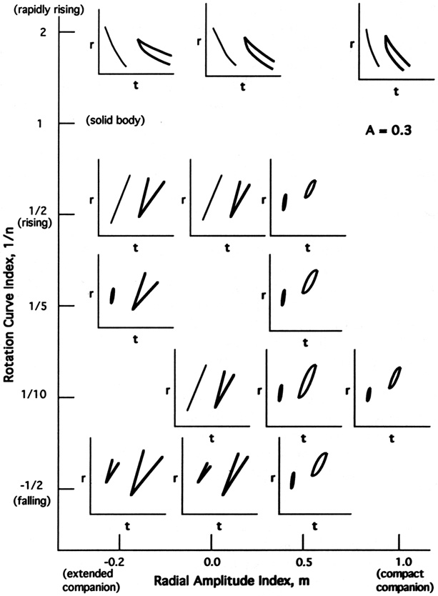
The success of the kinematic caustics theory is that the morphological variety of Figure 16 can be accounted for by the caustics Equation (4.13). This is demonstrated by Figure 17, which consists of a montage of the solutions of Equation (4.13) as a function of the parameters m, and n. In the low amplitude cases (e.g., A() 0.1) there are few caustic rings, although there will be significant orbit crowding, so these are not shown. Figure 17 shows the A() = 0.3 cases, i.e., relatively large amplitude cases. We will briefly consider some examples. First of all, in the m = 0 case the right-hand-side of Equation (4.13) is constant, so the phases t must also be independent of radius. Thus, one only has to solve Equation (4.13) once for the phases of the inner and outer ring edges. At any given time the Lagrangian radius of the edges can be determined from the equations t = constant, and then the Eulerian radii r(t) are given by Equation (4.5). This case was considered in detail in Struck-Marcell and Lotan (1990).

Figure 17. Schematic showing caustic borders of the first and second ring waves in radius-time plots as a function of the structural parameters m, n defined in the text. Specifically, thick lines or curves showing an inner and outer edge at any time represent caustic edges. A thinner, single line or curve represents an orbit-crowding region, without the orbit crossings that define a caustic region. The amplitude A = 0.3 is constant for all the figures in this assemblage. Individual cases are discussed in the text.

Next consider rings at relatively large radii (q >> ), when n > 1 (i.e., the rotation curve rises less steeply with radius than for solid body rotation). In this case the second term on the left-hand-side of Equation (4.13) will usually dominate, since the first term is less than or of the order of unity. Then we also require that cos(t) < 1, or (2p - 1)(/2) < t < (2p + 1)(/2), for p = 1, 2, 3 .... In general, the first few rings will pinch off at radii that are not too large. In fact, Figure 17 shows that first ring caustics are rare, the first rings are usually weak.

If n < 0, the primary disk has a declining rotation curve. In this case the absolute value of the (1/n - 1) term is greater than in the rising rotation curve case, and rings tend to be more robust and broader. Physically this is simply because this case is still farther from the solid body case, and the orbital dispersion is correspondingly greater. When 0 < n < 1, the rotation curve rises more steeply than the solid body case and the rings propagate inward. To achieve this, the mass distribution would have to rise extremely rapidly with radius, for example if the galaxy contained a central deficiency of matter.

If m < 0, then the perturbation amplitude increases outward. Normally this is not physically realistic unless the "companion" is larger than the ring galaxy. In this case outward propagating rings become very broad with time.

Figure 17 also provides information on ring propagation speeds through the disk. Rings in disks with flat rotation curves tend to have a nearly constant propagation velocity. This is often assumed in estimates of ring ages from measured expansion velocities.

To summarize, several generalizations can be derived from Figure 17 and Equation (4.13).

1. Broad stellar rings result from declining rotation curves, or large amplitude perturbations. Thus, in cases with modest companions we suspect that the former is usually true. This seems to be the case in the "Sacred Mushroom", AM 1724-622 (see Wallin and Struck-Marcell 1994).

2. Widely spaced narrow rings occur in disks with flat or rising rotation curves. This is confirmed in the case of the Cartwheel (Higdon 1993; Struck-Marcell and Higdon 1993).

3. The variation of the velocity perturbation with radius determines (in part) the annular zone where caustic rings can occur, but this variation generally cannot be determined observationally.