


4.2. Luminosity Functions
In this section, we compare the detected EBL with the EBL predicted by luminosity functions measured as a function of redshift. To avoid unnecessary complications in defining apparent magnitude cut-offs, and to facilitate comparison with other models of the luminosity density as a function of redshift, we compare luminosity functions with the total EBL rather than with EBL23, as in the previous section. To do so, we combine the EBL23 flux measured in Paper I with the flux from number counts at brighter magnitudes, as given in Table 2. Systematic errors in photometry of the sort discussed in Section 4.1 are likely to be relatively small for redshift surveys because the objects selected for spectroscopic surveys are much brighter than the limits of the photometric catalogs (although see Dalcanton 1998 for discussion of the effects of small, systematic photometry errors on inferred luminosity functions). We have not tried to compensate for such effects here.
The integrated flux from galaxies at all redshifts is given by
| (1) |
in which Vc(z) is the comoving volume element,
DL(z) is the luminosity distance,
 0 is the
observed wavelength, and
z =
0(1 +
z)-1 is the rest-frame wavelength at
the redshift of emission. To compare the detected EBL to the observed
luminosity density with redshift,
0 is the
observed wavelength, and
z =
0(1 +
z)-1 is the rest-frame wavelength at
the redshift of emission. To compare the detected EBL to the observed
luminosity density with redshift,
 (, z), we begin by
constructing the SED of the local luminosity density as a linear
combination of SEDs for E/S0, Sb, and Ir galaxies, weighted by their
fractional contribution to the local B-band luminosity density:
(, z), we begin by
constructing the SED of the local luminosity density as a linear
combination of SEDs for E/S0, Sb, and Ir galaxies, weighted by their
fractional contribution to the local B-band luminosity density:
| (2) |
in which the subscript i denotes the galaxy Hubble type (E/S0, Sb,
or Ir),
fi()
denotes the galaxy SED (the flux per unit
rest-frame wavelength), and
i(B,
0) is the B-band, local
luminosity density in ergs s-1 Å-1
Mpc-3. To produce
the integrated spectrum of the local galaxy population, we use
Hubble-type-dependent luminosity functions from
Marzke et al. (1998)
and SEDs for E, Sab, and Sc galaxies from
Poggianti (1997).
We adopt a local luminosity density of
B = 1.3
× 108
hL Mpc-3, consistent with the
Loveday et al. (1992)
value adopted by CFRS and also with
Marzke et al. (1998).
(1)
The spectrum we obtain for
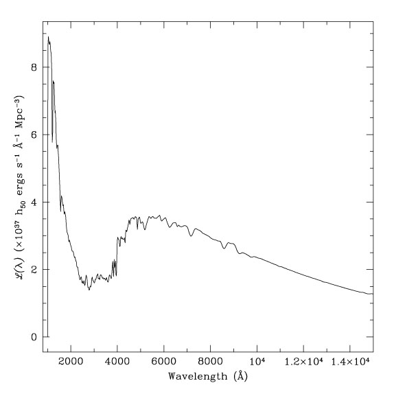
(, 0) is shown in
Figure 7.
Mpc-3, consistent with the
Loveday et al. (1992)
value adopted by CFRS and also with
Marzke et al. (1998).
(1)
The spectrum we obtain for
(, 0) is shown in
Figure 7.
|
Figure 7. The local luminosity density constructed by combining the spectral energy distributions of E/S0, Sab, and Sc galaxies weighted according to the type-dependent luminosity functions as described in Section 4.2 and Equation 2. |
We note that the recent measurement of the local luminosity function by Blanton et al. (2001) indicates a factor of two higher local luminosity density than found by previous authors. Previous results are generally consistent with Loveday et al. to within 40%. Blanton et al. attribute this increase to deeper photometry which recovers more flux from the low surface brightness wings of galaxies in their sample relative to previous surveys (see discussions in Section 4.1), and photometry which is unbiased as a function of redshift. For the no-evolution and passive evolution models discussed below, the implications of the Blanton et al. results can be estimated by simply scaling the resulting EBL by the increase in the local luminosity density. Although the Blanton et al. results do not directly pertain to the luminosity functions measured by CFRS at redshifts z > 0.2, they do suggest that redshift surveys at high redshifts will underestimate the luminosity density, as discussed by Dalcanton (1998).
In the upper panel of Figure 8, we compare the
EBL flux we detect with EBL flux predicted by five different models for
(, z), using the
local luminosity density derived in
Equation 2 as a starting point.
For illustrative purposes, the first model we plot shows the EBL which
results if we assume no evolution in the luminosity density with
redshift, i.e. (, z) =
(, 0). The
number counts themselves rule out a non-evolving luminosity density,
as has been discussed in the literature for over a decade;
inconsistency between the detected EBL and the no-evolution model is
just as pronounced. The predicted EBL for the no-evolution model is a
factor of 10 fainter than the detected values (filled circles). These
are 1.7 ,
2.1, and
2.2 discrepancies at
U300, V555 and
I814, respectively. More concretely, the
no-evolution prediction is at least a factor of 12 × , 4 × ,
and 3.7 × lower than the flux in individually resolved
sources at U300, V555 and
I814 (lower-limit arrows).
Note that the no-evolution model still underpredicts the EBL if we
rescale the local luminosity density to the
Blanton et al. (2001)
values. This model demonstrates the well-known fact that luminosity
density is larger at higher redshifts.
,
2.1, and
2.2 discrepancies at
U300, V555 and
I814, respectively. More concretely, the
no-evolution prediction is at least a factor of 12 × , 4 × ,
and 3.7 × lower than the flux in individually resolved
sources at U300, V555 and
I814 (lower-limit arrows).
Note that the no-evolution model still underpredicts the EBL if we
rescale the local luminosity density to the
Blanton et al. (2001)
values. This model demonstrates the well-known fact that luminosity
density is larger at higher redshifts.

|
Figure 8. The upper panel shows the
spectrum of the EBL calculated by
integrating the luminosity density over redshift (Equation
1) for constant luminosity density, passively evolving
luminosity density, and evolution of the form
|
The second model we plot in Figure 8 shows the
effect of passive evolution on the color of the predicted EBL. In this
model, we have used the
Poggianti (1997)
SEDs for galaxies as a
function of age for H0 = 50 km s-1
Mpc-1 and
q0 = 0.225. In the Poggianti models, stellar
populations are 2.2 Gyrs old at a z ~ 3. The resulting
(, z) is bluer than
the no-evolution model due to a combination of K-corrections and
increased UV flux for younger stellar populations. The passive
evolution model does provide a better qualitatively match to the SED
of the resolved sources (lower limits) and EBL detections (filled
circles); however, it is still a factor of 3 × less than the
flux at U300, and a factor of 2 × less than the
flux we recover from resolved sources at V555 and
I814. For the
adopted local luminosity density and Poggianti models, passive
evolution is therefore not sufficient to produce the detected
EBL. Again, the passive evolution adopted here still underpredicts the
EBL if we rescale the local luminosity density by a factor of two to
agree with the
Blanton et al. (2001)
value.
As a fiducial model of evolving luminosity density, we adopt the form
of evolution implied by the CFRS redshift survey
(Lilly et al. 1996,
hereafter CFRS) and Lyman-limit surveys of
Steidel et al.
(1999):
(, z) =
(, 0)(1 +
z) ()
over the range 0 < z < 1 and roughly constant luminosity
density at
1 < z < 4. The remaining three models shown in
Figure 8
test the strength of evolution of that form which is allowed by the
EBL detections. The hatch-marked region shows the EBL predicted for
values of () which represent the
± 1 range
found by CFRS for the redshift range 0 < z < 1. The value
of the exponent
() is indicated in the lower
panel of Figure 8, and the hatch-marked region
reflects the
uncertainty in the high redshift luminosity density due to the poorly
constrained faint-end slope of the luminosity functions. This
± 1 range of the
predicted EBL is consistent with the detected
EBL at U300, but is inconsistent with the EBL
detections at V555 and I814 at the
1 level of both model and
detections. It is, however, consistent with the integrated flux in
detected sources at V555 and I814.
()
over the range 0 < z < 1 and roughly constant luminosity
density at
1 < z < 4. The remaining three models shown in
Figure 8
test the strength of evolution of that form which is allowed by the
EBL detections. The hatch-marked region shows the EBL predicted for
values of () which represent the
± 1 range
found by CFRS for the redshift range 0 < z < 1. The value
of the exponent
() is indicated in the lower
panel of Figure 8, and the hatch-marked region
reflects the
uncertainty in the high redshift luminosity density due to the poorly
constrained faint-end slope of the luminosity functions. This
± 1 range of the
predicted EBL is consistent with the detected
EBL at U300, but is inconsistent with the EBL
detections at V555 and I814 at the
1 level of both model and
detections. It is, however, consistent with the integrated flux in
detected sources at V555 and I814.
To test the range of evolution allowed by the full
± 2 range
of the EBL detections, we can explore two possibilities: (1) stronger
evolution at 0 < z < 1, shown in
Figure 8; and (2) evolution continuing beyond
z = 1, shown in Figures 9,
10, and
11. Addressing the possibility of
constant luminosity density at z > 1, the
dashed line in the upper panel of Figure 8 shows the
EBL predicted by the 2
upper limit for () from
CFRS; the dot-dashed line corresponds to the value of
() required to obtain the
upper limits of the EBL
detections at all wavelengths. Note that the latter implies a value
for (4400Å, 1)
which is ~ 10 × higher than the
value estimated by CFRS. This result emphasizes that the
2
interval of the EBL detections span a factor of 4 in flux at
4400Å, and thus the allowed range in the luminosity density for
< 4400Å and 0
< z < 1 is similarly large. Also, for each
model in which the luminosity density is constant at z > 1,
less than
50% of the EBL will come from beyond z = 1 due to the combined
effects of K-corrections and the decreasing volume element with
increasing redshift (see Figure 10).
|
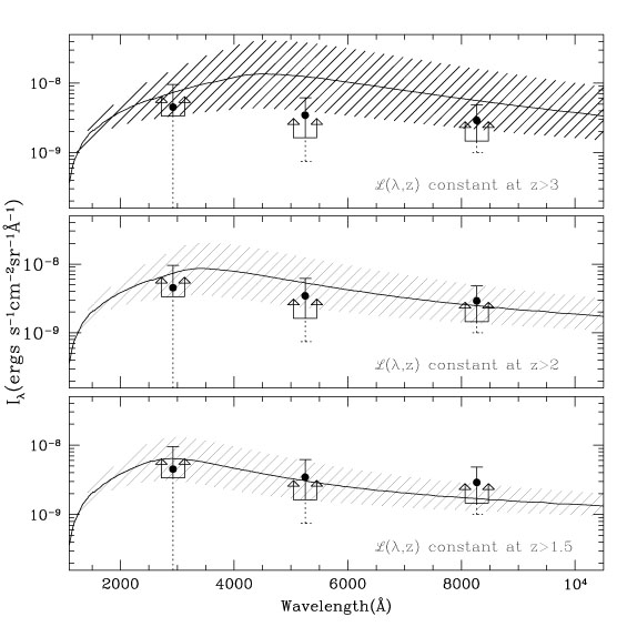
Figure 9. The three panels show the
spectrum of the EBL calculated assuming
|

|
Figure 10. The integrated EBL at
V555 contributed as a function of
increasing redshift from z = 0 to z = 10. As marked in
the figure, the lines show the
integrated flux for no evolution in the luminosity density,
passive evolution, and evolution of the form
|
Evolution continuing beyond z = 1 is possible if the
Lyman-limit-selected surveys have not identified all of the star
formation at high redshifts, and estimates of the luminosity density
at 3  z
4 are
subsequently low. Figures 9 and
10 show the EBL predicted
by models in which the luminosity density increases as (1 +
z)() to redshifts of
z = 1.5, 2 and 3. Clearly,
significant flux can come from z > 1 if the luminosity density
continues to increase as a power law. The rest-frame U300
luminosity density is plotted as a function of redshift in
Figure 11 for limiting values of the cut-off
redshift for evolution and
(). Although the strongest
evolution
plotted over-predicts the detected EBL, our detections are clearly
consistent with some of the intermediate values of the
() and increasing luminosity
density beyond z = 1.
For example, the mean rate of increase in the luminosity density found
by CFRS can continue to redshifts of roughly 2.5-3 without
over-predicting the EBL.
z
4 are
subsequently low. Figures 9 and
10 show the EBL predicted
by models in which the luminosity density increases as (1 +
z)() to redshifts of
z = 1.5, 2 and 3. Clearly,
significant flux can come from z > 1 if the luminosity density
continues to increase as a power law. The rest-frame U300
luminosity density is plotted as a function of redshift in
Figure 11 for limiting values of the cut-off
redshift for evolution and
(). Although the strongest
evolution
plotted over-predicts the detected EBL, our detections are clearly
consistent with some of the intermediate values of the
() and increasing luminosity
density beyond z = 1.
For example, the mean rate of increase in the luminosity density found
by CFRS can continue to redshifts of roughly 2.5-3 without
over-predicting the EBL.
|
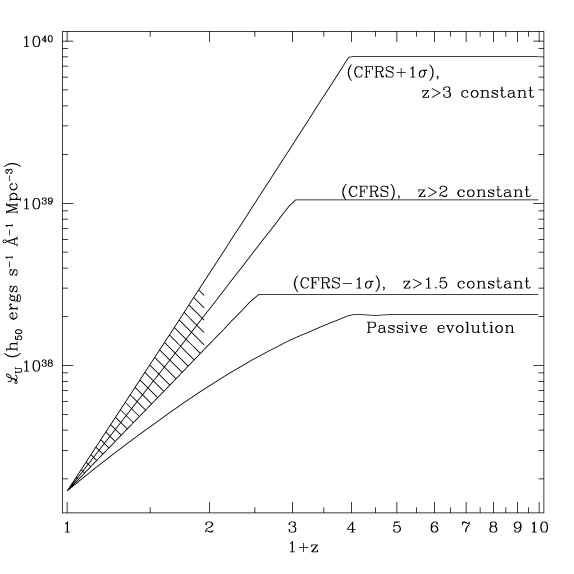
Figure 11. The luminosity density at
U300 as a function of redshift
corresponding to limiting cases plotted in
Figure 9.
The hatch-marked region indicates the
± 1 |
In all models, we have adopted the same cosmology (h = 0.5 and
 = 1.0) as assumed
by CFRS and
Steidel et al. (1999)
in calculating
(, z) and
(). Although the
luminosity density inferred from these redshift surveys depends on the
adopted cosmological model, the flux per redshift interval is a
directly observed quantity. The EBL is therefore a directly observed
quantity over the redshift range of the surveys, and is also
model-independent. To the degree that the luminosity density becomes
unconstrained by observations at higher redshifts, the EBL does depend
on the assumed (not measured) luminosity density and on the adopted
cosmology through the volume integral. Although dependence of the
predicted EBL on H0 cancels out between the luminosity
density, volume element, and distance in Equation 1,
H0 has some impact through cosmology-dependent time
scales, which
affect the evolution of stellar populations. If the luminosity
density is assumed to be constant for z > 1, the predicted EBL
increases by 25% at V555 for
(M = 0.2,
= 1.0) as assumed
by CFRS and
Steidel et al. (1999)
in calculating
(, z) and
(). Although the
luminosity density inferred from these redshift surveys depends on the
adopted cosmological model, the flux per redshift interval is a
directly observed quantity. The EBL is therefore a directly observed
quantity over the redshift range of the surveys, and is also
model-independent. To the degree that the luminosity density becomes
unconstrained by observations at higher redshifts, the EBL does depend
on the assumed (not measured) luminosity density and on the adopted
cosmology through the volume integral. Although dependence of the
predicted EBL on H0 cancels out between the luminosity
density, volume element, and distance in Equation 1,
H0 has some impact through cosmology-dependent time
scales, which
affect the evolution of stellar populations. If the luminosity
density is assumed to be constant for z > 1, the predicted EBL
increases by 25% at V555 for
(M = 0.2,
 = 0)
and corresponding values of
(), and decreases by 50%
for (0.2,0.8). The luminosity densities corresponding to the
2 upper limit of the
detected EBL change by the same fractions for the different cosmologies if
is constant at
z > 1. Similarly, for models in which the luminosity density
continues
to grow at z > 1, the luminosity density required to produce
the EBL will be smaller if we adopt (0.2,0) than (1,0), and smaller
still for (0.2,0.8). The exact ratios depend on rate of increase in the
luminosity density.
= 0)
and corresponding values of
(), and decreases by 50%
for (0.2,0.8). The luminosity densities corresponding to the
2 upper limit of the
detected EBL change by the same fractions for the different cosmologies if
is constant at
z > 1. Similarly, for models in which the luminosity density
continues
to grow at z > 1, the luminosity density required to produce
the EBL will be smaller if we adopt (0.2,0) than (1,0), and smaller
still for (0.2,0.8). The exact ratios depend on rate of increase in the
luminosity density.
Several authors
(Treyer et al. 1998,
Cowie et al. 1999,
and Sullivan et al.
2000)
have found that the
at UV wavelengths
(2000-2500Å) is higher than claimed by CFRS (2800Å) in the range
0 < z < 0.5 and have found weaker evolution in the UV
luminosity density, corresponding to
(2000Å) ~ 1.7. The
implications for the predicted EBL can be estimated from the plots of the
(U300,
z) shown in Figure 11, and the
corresponding EBL in Figures 9 and
10. For instance, if the local UV luminosity
density is a factor of 5 higher than the value we have adopted
and if (2000Å) ~
1.7 over the range 0 < z < 1, then the
rest-frame UV luminosity density at z = 1 is similar to that measured
by CFRS, and the predicted U300 EBL will be roughly
3.5 × 10⁻⁹ cgs, very similar to the EBL we derive from
our modeled local luminosity density and the mean values for
() from CFRS.
1 For a
B-band solar irradiance of
L = 4.8
× 1029ergs s-1 Å-1,
(B, 0) = 6.1
× 1037h ergs s-1 Mpc
-3 = 4.0 × 10¹⁹h50 W
Hz-1 Mpc-3.
Back.
 (1 +
z)
(1 +
z)