6. MAXIMUM-LIKELIHOOD ERROR, ONE PARAMETER

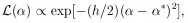
It can be shown that for large N, () approaches a Gaussian distribution. To this approximation (actually the above example is always Gaussian in ), we have

where 1 / h is the rms spread of about *,

Since as defined in Eq. (3) is 1 / h , we have

(7)

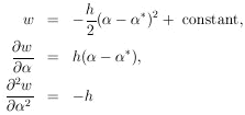
It is also proven in Cramer [4] that no method of estimation can give an error smaller than that of Eq. 7 (or its alternate form Eq. 8). Eq. 7 is indeed very powerful and important. It should be at the fingertips of all physicists. Let us now apply this formula to determine the error associated with * in Eq. 6. We differentiate Eq. 5 with respect to . The answer is

Using this in Eq. 7 gives

This formula is commonly known as the law of combination of errors and refers to repeated measurements of the same quantity which are Gaussian-distributed with "errors" _i.

In many actual problems, neither * nor may be found analytically. In such cases the curve () can be found numerically by trying several values of and using Eq. (2) to get the corresponding values of (). The complete function is then obtained by drawing a smooth curve through the points. If () is Gaussian-like, ð²w / ð² is the same everywhere. If not, it is best to use the average

A plausibility argument for using the above average goes as follows: If the tails of () drop off more slowly than Gaussian tails, is smaller than

Thus, use of the average second derivative gives the required larger error.

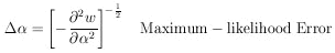
Note that use of Eq. 7 for depends on having a particular experimental result before the error can be determined. However, it is often important in the design of experiments to be able to estimate in advance how many data will be needed in order to obtain a given accuracy. We shall now develop an alternate formula for the maximum-likelihood error, which depends only on knowledge of f (; x). Under these circumstances we wish to determine averaged over many repeated experiments consisting of N events each. For one event we have

for N events

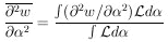
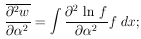
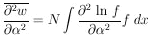
This can be put in the form of a first derivative as follows:

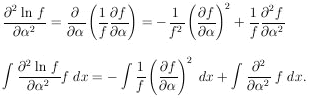
The last integral vanishes if one integrates before the differentiation because

Thus

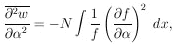
and Eq. (7) leads to

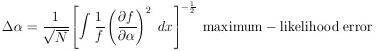
(8)

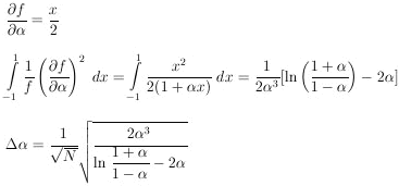
Example 1

Assume in the µ-e decay distribution function, f (; x) = (1 + x) / 2 , that ₀ = - 1/3. How many µ-e decays are needed to establish a to a 1% accuracy (i.e., / = 100)?

Note that

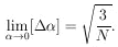
For

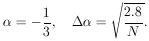
For this problem