


Cross-correlation analysis is the tool most commonly used in the analysis of multiple time series. Because its application to astronomical time series is often misunderstood and has historically been rather contentious, it merits special attention. Important steps in the development of cross-correlation analysis as applied to AGN variability studies can be found in the literature 27, 28, 20, 49, 39 .

|
Figure 22. The left-hand panel shows
simultaneous measurements
of H |
Cross-correlation analysis is basically a generalization of standard
linear correlation analysis, which provides us with a good place to
start. Suppose we obtain repeated spectra of one of the brighter
Seyfert galaxies, and we want to determine whether or not the
variations in the H emission
line and the optical continuum
are correlated (which was an interesting question 20 years ago,
even before emission-line time delays were considered).
The first thing you would do is plot the
H flux against the
continuum flux, as in the left-hand
panel of Fig. 22, which shows that the two
variables are indeed correlated. A measure of the strength of the
correlation is given by the correlation coefficent,
emission
line and the optical continuum
are correlated (which was an interesting question 20 years ago,
even before emission-line time delays were considered).
The first thing you would do is plot the
H flux against the
continuum flux, as in the left-hand
panel of Fig. 22, which shows that the two
variables are indeed correlated. A measure of the strength of the
correlation is given by the correlation coefficent,
| (31) |
where there are N pairs of values (xi,
yi) and their respective
means are  and
and
 . When the two variables
x and
y are perfectly correlated, r = 1. If they are perfectly
anticorrelated,
r = -1. If they are completely uncorrelated, r = 0. For
the data shown in the left panel of
Fig. 22, r = 0.596; for 24 pairs of
points, as shown
here, this means that the correlation is significant at the
. When the two variables
x and
y are perfectly correlated, r = 1. If they are perfectly
anticorrelated,
r = -1. If they are completely uncorrelated, r = 0. For
the data shown in the left panel of
Fig. 22, r = 0.596; for 24 pairs of
points, as shown
here, this means that the correlation is significant at the
 99.8% confidence
level (i.e., the chance that the two variables are
in fact completely uncorrelated and the correlation we find is
spurious is less than 0.02%. Confidence levels for linear correlation
can be found in standard statistical tables
6).
99.8% confidence
level (i.e., the chance that the two variables are
in fact completely uncorrelated and the correlation we find is
spurious is less than 0.02%. Confidence levels for linear correlation
can be found in standard statistical tables
6).
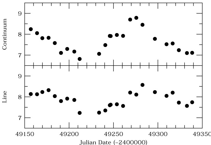
While this is quite a good correlation, we see something more remarkable if we plot both variables as functions of time (i.e., as light curves), as seen in Fig. 23. We see that the patterns of variation are very similar, except that the emission-line light curve is delayed in time, or "lagged," relative to the continuum light curve. It is obvious that the correlation between the continuum and emission-line fluxes would be even better if we allowed a linear shift in time between the two light curves in order to line up their prominent maxima and minima. This is what cross-correlation does.
|
Figure 23. The
H |
The first operational problem in computing a cross-correlation is
also immediately apparent: since each point in one light curve must
be paired with a point in the other light curve, it is obvious that
the data should be regularly spaced. The cross-correlation is then
evaluated as a function of the spacing between the
interval between data points
 t using the pairs
[x(ti), y(ti +
Nt)] for all
integers N.
Unfortunately, regularly sampled data are almost never found in Astronomy;
ground-based programs have weather to contend with, and even
satellite-based observations are almost never regularly spaced in time.
The essence of the cross-correlation problem in Astronomy is dealing with
time series that are not evenly sampled. Moreover, the light
curves are often limited in extent and are noisy.
t using the pairs
[x(ti), y(ti +
Nt)] for all
integers N.
Unfortunately, regularly sampled data are almost never found in Astronomy;
ground-based programs have weather to contend with, and even
satellite-based observations are almost never regularly spaced in time.
The essence of the cross-correlation problem in Astronomy is dealing with
time series that are not evenly sampled. Moreover, the light
curves are often limited in extent and are noisy.
For well-sampled
series as in Fig. 23, the sampling problem can be
dealt with in a straightforward fashion. The simple, effective solution
is to interpolate one series between the actual data points, and
use the interpolated points in the cross-correlation. We illustrate
this schematically in Fig. 24. We can then
compute the cross-correlation function
CCF( ),
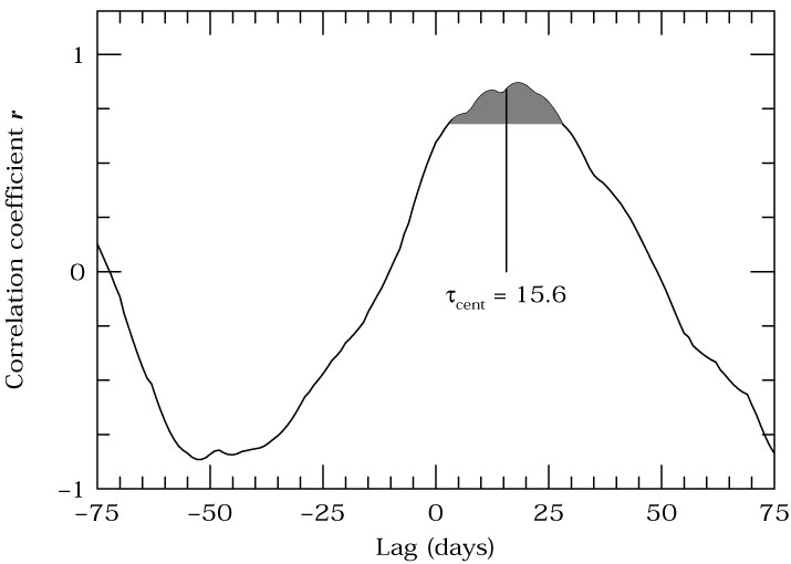
as shown in Fig. 25, and
the step size we use for is now
somewhat arbitrary.
At each value of the lag we
compute r as in Eq. (31).
For the example we have been using, we find that the
CCF is maximized when points in the continuum light curve are
matched to those in the emission-line light curve with a delay
of 15.6 days. If we plot the shifted emission-line
values versus the continuum values (as we have done in the
right-hand panel of Fig. 22)
and again perform a linear correlation analysis, we find
that the fit has improved, with r = 0.849 and
),
as shown in Fig. 25, and
the step size we use for is now
somewhat arbitrary.
At each value of the lag we
compute r as in Eq. (31).
For the example we have been using, we find that the
CCF is maximized when points in the continuum light curve are
matched to those in the emission-line light curve with a delay
of 15.6 days. If we plot the shifted emission-line
values versus the continuum values (as we have done in the
right-hand panel of Fig. 22)
and again perform a linear correlation analysis, we find
that the fit has improved, with r = 0.849 and

 2 = 1.76.
|
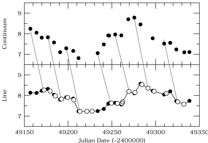
Figure 24. Continuum and emission-line light curves for Mrk 335, as in Fig. 23. This illustrates the interpolation method commonly used in cross-correlation. In this figure, the emission-line light curve is made continuous through linear interpolation between data points. Actual continuum observations are then paired with interpolated emission-line values to compute the correlation coefficient for a particular time delay. In this example, we show interpolated emission-line fluxes that are time-delayed relative to the continuum by 15.6 days, which is the value at which the cross-correlation function peaks. As a visual aid, dotted lines join a few of the data pairs. Notice how the first few points of the emission-line series and the last few points of the continuum series remain unused. |
|
Figure 25. The interpolation
cross-correlation function for
the Mrk 335 data shown in the previous figures.
The shaded area indicates points with values
r |
 0.8rpeak, which are the points used in computing
the centroid, which is also indicated.
0.8rpeak, which are the points used in computing
the centroid, which is also indicated.