6. UNBIASED SFR ESTIMATORS

The central result we have found is that the extinction correction including the effects of an underlying stellar Balmer absorption brings into agreement all four SFR estimators, and that the photon escape correction seems to play a minor role.

We have seen that the SFR given by the UV continuum is equal to the SFR given by the FIR if the extinction correction is estimated using the Calzetti extinction curve and including the underlying Balmer absorption corrections. It is reassuring that the simple inclusion of the underlying absorption correction brings into agreement theory and observations. We have used the results from the previous sections to obtain SFR estimators that are free from these systematic effects,

(12)

where the SFR(H) is obtained from the reddening corrected H luminosity while the expressions for the SFR(OII) and the SFR(UV) are for the observed fluxes.

These estimators, (the SFR(OII) and the SFR(UV) from equation 12) should be applied to samples where it is not possible to determine the extinction. If the objects have similar properties to our selected sample, then any systematic difference between the different estimators should be small.

We have applied this new set of calibrations to the SFR values given by different authors at different redshifts: Gallego et al. (1995) H survey for the local Universe, Cowie et al. (1995) [OII]3727 sample and Lilly et al. (1995) UV continuum one between redshifts of 0.2 and 1.5 and Connolly et al. (1997) between 0.5 and 2; and the UV points by Madau et al. (1996) and Steidel et al. (1999) at redshift higher than 2.5. We give in Table 3 the complete list of surveys of star formation at different redshifts that we have used plus their different tracers and computed SFR.

Table 3. SFR for surveys at different redshifts. The mean luminosity density () is given in units of erg s^-1Mpc^-3 for the case of the H and OII emission lines and the FIR. The UV is given in erg s^-1Hz^-1Mpc^-3. The SFR referred to as standard are given by the expressions by Kennicutt (1998) and described in Section 3. The SFR referred to as unbiased are the ones obtained by using Equation 12. In both cases, the SFR are given in units of M yr^-1 Mpc^-3.

Redshift	SFR	log ()	log(SFR)	log(SFR)	Log Error	References
Range	Tracer		(Standard)	(Unbiased)
0.0-0.045	H	39.09	-2.01	-1.87	0.2	[Gallego et al. 1995]
0.1-0.3	H	39.47	-1.63	-1.50	0.04	[Tresse & Maddox 1998]
0.75-1.0	H	40.22	-0.75	-0.88	0.17	[Glazebrook et al. 1999]
0.25-0.50	FIR	41.85	-1.50	-1.50	0.26	[Flores et al. 1999]
0.50-0.75	FIR	42.17	-1.18	-1.18	0.26	[Flores et al. 1999]
0.75-1.00	FIR	42.49	-0.86	-0.86	0.26	[Flores et al. 1999]
0.25-0.50	OII	38.83	-2.02	-1.24	0.1	[Cowie et al. 1995]
0.50-0.75	OII	39.12	-1.73	-0.95	0.1	[Cowie et al. 1995]
0.75-1.00	OII	39.39	-1.46	-0.68	0.1	[Cowie et al. 1995]
1-1.25	OII	39.25	-1.60	-0.82	†	[Cowie et al. 1995]
1.25-1.50	OII	39.21	-1.64	-0.86	†	[Cowie et al. 1995]
0.25-0.50	UV	25.89	-1.96	-1.30	0.07	[Lilly et al. 1996]
0.50-0.75	UV	26.21	-1.64	-0.98	0.08	[Lilly et al. 1996]
0.75-1.00	UV	26.53	-1.32	-0.66	0.15	[Lilly et al. 1996]
0.4-0.7	FIR	42.64	-0.76	-0.76	(+0.1)(-0.2)	RR97
0.7-1.0	FIR	43.23	-0.13	-0.13	(+0.4)(-0.2)	RR97
0.5-1.0	UV	26.52	-1.33	-0.63	0.15	[Connolly et al. 1997]
1.0-1.5	UV	26.69	-1.16	-0.50	0.15	[Connolly et al. 1997]
1.5-2.0	UV	26.59	-1.26	-0.60	0.15	[Connolly et al. 1997]
2.0-4.0	FIR	42.80	-0.85	-0.85	†	[Hughes et al. 1998]
2.0-3.5	UV	26.42	-1.43	-0.77	0.15	[Madau et al. 1996]
3.5-4.5	UV	26.02	-1.83	-1.17	0.2	[Madau et al. 1996]
2.8-3.3	UV	26.28	-1.57	-0.91	0.07	[Steidel et al. 1999]
3.9-4.5	UV	26.19	-1.66	-1.00	0.1	[Steidel et al. 1999]

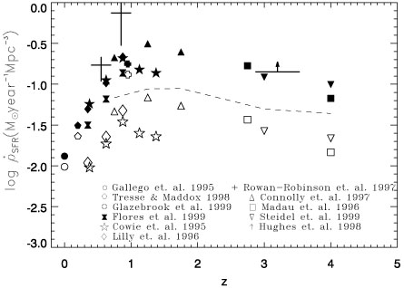
The results are plotted in Figure 9. We have also plotted the results obtained by Hughes et al. (1998) based on SCUBA observations of the Hubble Deep Field, those by Chapman et al. (2001) based on sub-millimeter observations of bright radio sources and those by Rowan-Robinson et al. (1997) based on observations at 60 µm of the Hubble Deep Field. Clearly the mm/sub-mm results and our "unbiased" results agree within the errors. The "unbiased" history of star formation is characterized by a large increase of the SFR density from z ~ 0 to z ~ 1 (a factor of about 20) and a slow decay from z ~ 2 to z ~ 5.

Figure 9. The SFR density as a function of redshift. The solid and open symbols represent values corrected and uncorrected for reddening respectively, except for the H values (the two lowest z points) which are all reddening corrected. The SFR in all cases are estimated using equations 2, 3, 4 and 5 for open symbols and equations 12 for the filled symbols. The open circle is the SFR based on H emission line corrected by extinction from Gallego et al. (1995) sample. The open stars are the SFR determined by [OII]3727 from the sample of Cowie et al. (1995) without any correction. The UV continuum samples are from Connolly et al. (1997) (triangles) Madau et al. (1996) (squares) and Steidel et al. (1999) (upside down triangles). The upward arrow is the lower limit given by Hughes et al. (1998) based on sub-mm observations of the Hubble Deep Field. The crosses at z = 0.55 and 0.85 correspond to the SFR estimates by Rowan-Robinson et al. (1997). The dashed line is the lower limit given by Chapman et al. (2001)

The final corrected values are similar to other published results (e.g. Somerville, Primack and Faber 2001). But the fact that our procedure removes systematic (or zero point) differences between the different estimators, implies that the shape of the curve, and therefore the slopes between z = 0 and 1 and z = 1 and 4 are now better determined.