Copyright © 1988 by Annual Reviews. All rights reserved
| Annu. Rev. Astron. Astrophys. 1988. 26:
561-630 Copyright © 1988 by Annual Reviews. All rights reserved |


4.1. The Predicted Hubble Diagram With No Luminosity
Evolution
The N(z, q0) volume-redshift relation of
the last section is very
difficult to apply in practice because complete galaxy counts in
redshift space require redshift measurements of every galaxy (of all
types and surface brightness) in the volume, or else a correction for
sample incompleteness in a redshift survey that is complete to a given
magnitude limit
(Loh & Spillar 1986,
Loh 1986).
These corrections must
be highly precise if the small differences in the N(m,
q0) curves in
Figure 1 are to be measured. For this reason, the value of
q0 via this
route is quite uncertain at the moment.
The easier test observationally is the count-magnitude relation,
N(m, q0), used in its most elementary
form by Hubble (1936b),
following the theory set out by
Hubble & Tolman (1935)
for N(r). We
now cast their discussion into modern form by using the closed
equation for the apparent magnitude-redshift relation via the Mattig
equations and thereby changing N(z, q0)
into the N(m, q0) count-magnitude
prediction.
The apparent bolometric flux fb received at Earth from
a galaxy
receding with redshift z whose absolute flux (at the source) is
Fb was shown by
Robertson (1938)
(after some debate) to be
For an appreciation of this equation, consider a sphere of interval
radius l (Equations 12, 13) centered on the source, over which
the flux
of a light pulse is spread at the time of light reception,
t0, at the Earth. The area of this sphere is not
4
The difference in the area compared with the Euclidean case is
accounted for in Equation 32 by the
(R0r)2 factor rather than by
simply using the interval distance l, which would be incorrect. The
(1 + z)2 term accounts for the energy depletion and
dilution factors of
the radiation due to the redshift. One factor arises because each
photon is decreased in energy by (1 + z), and hence the entire
ensemble
is depleted by the same factor. The second factor of (1 + z) is
present
if the redshift is due to true expansion. It is caused by the
increased path length, with the consequent decrease in the energy
density. If the Universe is not expanding, the second (1 +
z) factor
would not be present, a crucial point for the surface brightness test
discussed in Section 8.
Converting Equation 32 into magnitudes and using Equation 30 for
(R0r)2 gives the theoretical
m(z, q0) equation for the Hubble
diagram in terms of the bolometric magnitude:
where the constant C is
2.5 log 4
Series expansion of Equation 33 gives the well-known equation (e.g.
Robertson 1955,
McVittie 1956)
used by Humason et al.
(1956;
hereinafter HMS) in their early analysis
of cluster data. Although adequate to z ~ 0.3, the deviations of
Equation 34 from Equation 33 for larger z become inadequately large
(cf. Mattig 1958,
his Figure 1).
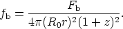
(32)
 l2 if the
geometry is non-Euclidean but is, rather,
4(R0r)2, where
R0r = R0sin l /R
using
Equation 12 for k = + 1. As in the case of the spherical cap of
Equation 5, this area is smaller than
4l2 owing to
the spatial curvature if k = + 1, or larger if k = - 1:
l2 if the
geometry is non-Euclidean but is, rather,
4(R0r)2, where
R0r = R0sin l /R
using
Equation 12 for k = + 1. As in the case of the spherical cap of
Equation 5, this area is smaller than
4l2 owing to
the spatial curvature if k = + 1, or larger if k = - 1:

(33)
+ 5 log
c/H0. Note that the factor
(1 + z)2 of Equation 32 is incorporated in Equation 33
as part of the
theory. Some earlier writers, following Hubble, included the
-5 log(1 + z) factor as a correction term to the observed
magnitudes (as
part of a generalized K term). This is not the modem practice,
however, which, as done here, carries this factor into Equation 33 via
Equation 32. This point is very important if the reader is to
understand
Hubble's (1936b)
method of correction, which differs
fundamentally from the modem practice, based on the equations given here.

(34)