4.4. Individual and Orbital Masses of Double Galaxies

A remarkable observational discovery in the dynamics of galaxies in recent years has been the identification of non-Keplerian rotation in the peripheral regions of many galaxies (Shostak and Rogstead, 1973). The prevalence of such flat rotation curves was convincingly demonstrated by Rubin and her collaborators (1980, 1982). The constancy of rotational velocity V(R) to the optical edge of the galaxies, contrasted with the asymptotic Keplerian behaviour V ~ R^-1/2 for a point mass, indicates the presence of invisible massive haloes around these galaxies. The maximal extent and total mass of the postulated circumgalactic haloes are almost unknown because of the obvious difficulty of measuring V(R) beyond the optical edge of the galaxies. We work around this difficulty by a different method, measuring the masses of galaxies from their orbital motions in isolated pairs in which the separation between components generally exceeds their apparent sizes. However, the mean orbital mass-to-luminosity ratio <f₀> = 7.75 obtained in section 4.2 for double galaxies may be accounted for without any additional assumptions about invisible massive haloes. This apparent contradiction between two solid observational results deserves the most careful attention.

The proper resolution of this contradiction may be reached by comparing the orbital estimates of masses with the sum of the masses determined from internal motions for pair members. Such an approach has been presented earlier (Karachentsev, 1974, Dickel and Rood, 1980, van Moorsel, 1983), but the small number of cases studied in comparison with the number required for a proper statistical investigation of the problem did not allow a clear result. There currently exists a large number of galaxies located in pairs for which individual masses have been measured from rotation curves, from profile widths of the 21-cm radio HI line, or from the velocity dispersion of stars around the nuclear region of the galaxy. Karachentsev (1985) attempted to put all of these results into a single uniform system, incorporating the three different ways of looking at the observational data.

1. The most direct calculation of the mass is based on measuring the rotation curve of a galaxy. For a model with a spherical distribution of mass contained within some specified radius R, the rotation curve has the form

(4.36)

where G is the gravitational constant. In the case of a flat rotation curve (V = constant), the mass increases linearly with radius, which may be described as saying that each R yields a distinct estimate of the mass. We will use the mass estimate corresponding to material within the standard isophote 25^m/sq.arc sec.

(4.37)

where V_m is the maximum rotation velocity in the galaxy and A₂₅ is the linear diameter at the chosen isophote. With this technique we can obtain masses for 32 components of pairs. The basic data here are from our observations (Karachentsev and Mineva, 1984b). For five objects (double galaxies 27ab, 355ab, and 603a), estimates of V_m were taken from the works of Rubin and Ford (1983) and the Burbidges (1961, 1963). Note that for galaxies of late structural type it is important to include a thin disk in the model. This reduces the mass by 30% compared to a spherical model. For the moment we have ignored these distinctions.

2. Thanks to the work of Fisher and Tully (1981) and other observers, the line profile of the 21-cm HI line, W_p, has been measured for several thousand spiral galaxies. Among these are 126 galaxies located in pairs of our catalogue. For galaxies whose angular diameter does not exceed the beam width of the radio telescope, the maximum rotational velocity may be obtained using the calibration presented by Fisher and Tully (1981)

(4.38)

where W₂₀ is the width of the HI profile at 20% of maximum intensity, and i is the angle of inclination of the axis of rotation to the line of sight. To get the masses M₂₅ in (4.37) we used the estimates of W₂₀ presented by Fisher and Tully (1981). The system was augmented by further data from Hoffmeier et al. (1983), in which we compared estimates of the line width at heights of 20% and 25%. For several galaxies with measured W_p at the 50% level we used the empirical relation <W₂₀ > = 1.38 <W₅₀>. The inclination of galaxies was determined from cos i = (b/a)₂₅, where (b / a)₂₅ is the axial ratio reduced to the standard isophote. This method has several limitations. For small values of i, errors in measuring the angle of inclination introduce non-negligible errors in the mass estimator. For close pairs it is possible to include both components in the measurement and measure a line profile coming simultaneously from both galaxies. Further, Lewis (1983) showed that for galaxies with narrow lines there is a tendency to overestimate the width of the line because of statistical fluctuations. This happens most often in estimates for galaxies of late types, of generally low luminosity. Finally, this method is inapplicable to the vast number of galaxies of early type, which are gas poor.

3. In recent years a very extensive sample of galaxies has emerged for which the mass can be estimated from the stellar velocity dispersion s_V² in the central regions of the galaxy. From the virial energy balance for galaxies with a density distribution following a de Vaucouleurs law, an estimate of the total mass is

(4.39)

where A_e is the effective linear diameter within which half of the luminosity (or mass) of the galaxy is found, and the coefficient _e = 0.3358 (Poveda, 1958) is characteristic of a de Vaucouleurs profile. The dimensionless factor k incorporates the integration of the measured velocity dispersion along the radius of the galaxy. According to the data presented by Tonry (1983) we adopt k = 1/2. The effective diameter A_e is known for only a small number of galaxies. For 194 galaxies from the RCBG we have the mean relation

(4.40)

which will be used to determine mass within the standard isophotal diameter of the galaxy A₂₅. The term c_T in (4.40) incorporates a weak dependence on morphological type. Empirical values for this correction are: 0.00 (E), +0.06 (S0), +0.03 (Sa), -0.02 (Sb) and -0.05 (Sc). Therefore, the equivalent of (4.39) will be

(4.41)

In the work of Tonry and Davis (1981) and White et al. (1983) measurements of s_V are given for 69 galaxies in common with our catalogued pairs. We have incorporated these mass estimates. The bulk of the galaxies in this last sample occur among the early types E and S0 which somewhat compensates for the selection bias of the first two methods.

Altogether, the three methods give measurements of the individual masses for 227 galaxies in pairs. In the calculation by Karachentsev (1985) there were 119 pairs included for which individual masses were known either for both components or for the brighter one, when its luminosity exceeds 60% of the total luminosity of both pair members. That calculation also includes mass estimates for 35 components of double systems, the luminosity of which does not satisfy this lower limit. For such galaxies, individual mass-to-luminosity ratios f_in were calculated. Comparison of the mean values grouped according to the three methods show that the various methods yield results which are the same to within the expected statistical errors.

The overall distribution of 227 double galaxies according to their individual mass-to-luminosity ratios is shown in figure 26. It has an asymmetric appearance, close to a log-normal form, agreeing very well with the data of Shaw and Reinhart (1973). The mean value of f_in is 7.3 ± 0.4 with standard deviation _f = 5.0. It is important to note here that <f_in> for the components of pairs agrees very well with the analogous mean for isolated galaxies <f_ig> = 7.0 ± 1.0 (Karachentsev and Mineva, 1984a), and further with the uncontaminated mean estimate of orbital mass-to-luminosity ratio 7.8 ± 0.7 obtained from a sample of 286 pairs (see table 8).

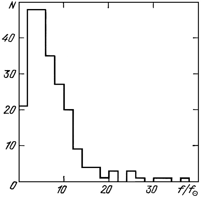Figure 26.

In section 3.6 it was demonstrated that the luminosities of galaxies in pairs are tightly correlated with one another. An analogous empirical relation also appears for the individual masses of double galaxies. For 73 pairs the correlation coefficient for log M for the two components is +0.68, with 95% confidence interval [0.52 - 0.81]. Part of this effect, obviously, arises from observational selection. In contrast to masses or luminosities, their ratio f_in should not depend on the basic selection of double systems. Nevertheless, figure 27 demonstrates a much weaker correlation coefficient (+0.48) between log f_in for pair members. The mutual association of mass-to-luminosity ratios for double galaxies apparently arises from the basic formation of pair members from common protogalactic surroundings.

Figure 27.

We will begin with this empirical form, and, by extrapolating it, assume that the value of f_in is a constant for the components of pairs. This allows us to add to the 73 pairs with measured sums of individual galaxy masses, another 46 for which the mass of the fainter component is estimated from its luminosity. Therefore, we have a sub-sample of 119 pairs with orbital mass to total individual mass ratios

(4.42)

The distribution of values of logµ for 119 pairs is shown in figure 28. The logarithmic scale was chosen to include the entire range of logµ, more than six orders of magnitude. Analysing this distribution we focus attention on four basic effects which can introduce a large dispersion in µ:

a) fluctuations in the projection factor (4.8) and their effect on orbital mass;

b) the presence of false pairs in the sample examined;

c) measurement errors in the radial velocity which affect estimates of orbital mass;

d) possible presence within the chosen isophote A₂₅ of invisible mass, such as is required to explain flat rotation curves.

Figure 28.

1. Projection effects. If all of the mass of double systems were located within the optical boundaries of their components, the ratio of estimates of the orbital mass of the pair to the sum of the individual masses of the galaxies becomes identically equal to the projection factor (µ ). For circular orbits, the factor will be bounded in the interval [0, 32 / 3]. For the general case of elliptical motion with orbital eccentricity e, the interval of possible values of extends somewhat higher: [0, (1 + e)32 / 3]. Using a random realisation of (4.11) and (4.12) we modelled the distribution of log for various values of the eccentricity. Results for e = 0.05, 0.35, 0.65 and 0.95 are presented in figure 29. For pure circular motion, the distribution p (log) rises monotonically with increase in and peaks with a value log(32 / 3) 0.53. For the other values of orbital eccentricity, the peak of the distribution on the right side becomes less pronounced, and the maximum of the distribution drops and moves towards lower values of . The sensitivity of the form of the distribution p (log) to the value of the eccentricity allows determination of the type of orbital motion in the catalogue pairs. The best agreement with the observed distribution is for e = 0.25. The density distribution p (log) for e = 0.25 is shown in figure 28 as the curved line. Low values of eccentricity found in this way agree very well with the results presented in section 4.2.

Figure 29.

2. The role of fictitious pairs. The histogram in figure 28 presents the distribution in logµ of all double systems regardless of radial velocity difference or orbital mass-to-luminosity ratio. The information from the modelling (section 3.2), showed that around 44% of the objects in the catalogue would be non-isolated members of systems, or optical pairs. It is obvious that these false double systems have excessive values of µ in the region µ > 64 / 3. The relative number of cases in this critical region is only 21%, which allows a simple discrimination of these fictitious pairs.

We may introduce two pieces of evidence to support the notion that the tail of the distribution in figure 28 for µ > 64 / 3 consists of false pairs. Firstly, consider the pairs which satisfy the strictest isolation criterion (++). The relative number of fictitious pairs in this sub-sample should be less by an order of magnitude than in the whole sample. The strictly isolated double systems are shown with cross hatching in figure 28. Not one of these is in the critical region µ > 64/3.

The physical nature of double galaxies may also be shown by signs of interaction between them. Forty-eight pairs with known ratio µ exhibit tails, bridges, or a common atmosphere. Only two of these, numbers 481 and 483, have orbital mass to total galaxy mass ratios higher than the critical value. Both of these pairs are located in the central region of the large cluster in Hercules and their velocities are typical of the radial velocities found in this cluster. Most probably these are chance superpositions along the line of sight of cluster members which manage to imitate interacting pairs.

3. Errors in measured velocities. In calculating the orbital mass of pairs from (4.8) we incorporated the error _y in measuring the radial velocity difference. Because of the quadratic dependence of M on y, estimates of the orbital mass will be systematically high. The unbiased estimate of orbital mass uses M_c = (32 / 3) G^-1 X(y² - _y²). For large values of _y the quantities M_c and µ_C = M_c / (M₁ + M₂) may produce spurious values which will falsify the analysis of the observational data. The general effect of errors is to dilute the strong maximum of the distribution p (logµ) and increase the fraction of pairs in the critical region, µ > 64 / 3.

Calculation of all these effects shows that the observed distribution of pairs according to the value of µ may be explained without incorporating any massive invisible haloes around double galaxies. In view of the considerable importance of this question we will examine it further below.