


3.1. The two-point correlation function
The structure of the universe qualitatively described in the previous section needs to be quantified by means of statistical measures having the capacity of distinguish between different point patterns.
The most popular measure used in this context has been the
two-point correlation function
[14,
1]
 (r). The
first time this quantity was applied to a galaxy catalog was in
1969 by Totsuji and Kihara
[15].
Since then, its use has been widely spread. The quantity
(r) is
defined in terms of the
probability that a galaxy is observed within a volume dV lying
at a distance r from an arbitrary chosen galaxy,
(r). The
first time this quantity was applied to a galaxy catalog was in
1969 by Totsuji and Kihara
[15].
Since then, its use has been widely spread. The quantity
(r) is
defined in terms of the
probability that a galaxy is observed within a volume dV lying
at a distance r from an arbitrary chosen galaxy,
 |
(2) |
where n is the average galaxy number density. For a completely
random distribution
(r) =
0. Positive values indicate
clustering, negative values indicate anti-clustering or
regularity. In this definition, isotropy and homogeneity of the
point process is being assumed, otherwise the function
(r)
should depend on a vector quantity.
Several estimators have been used to obtain the two-point correlation function from a given data set [16, 17]. At short distances their results are nearly indistinguishable; at large distances, however, the differences become important. The best performance is reached by the Hamilton [18] and the Landy and Szalay [19] estimators.
To illustrate the kind of information that we can extract from
this second-order spatial statistic we can use a point process
having an analytic expression for its two-point correlation
function. A segment Cox process is generated by randomly placing
segments of length  within a
window W. Then, we scatter
points on the segments with a given intensity. If the mean number
of segments per unit volume is
within a
window W. Then, we scatter
points on the segments with a given intensity. If the mean number
of segments per unit volume is
 s, the
correlation function of the process has the form
[20]
s, the
correlation function of the process has the form
[20]
 |
(3) |
for r  and vanishes for larger
r. Note that this
expression is independent of the number of points per unit length
scattered on each segment.
and vanishes for larger
r. Note that this
expression is independent of the number of points per unit length
scattered on each segment.
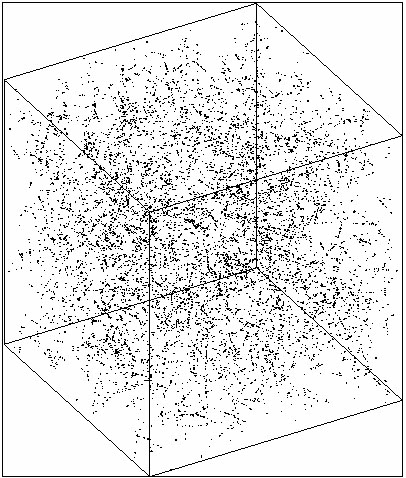
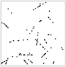
In Fig. 4 we show a 3-D simulation of this process
with parameters
s = 0.001
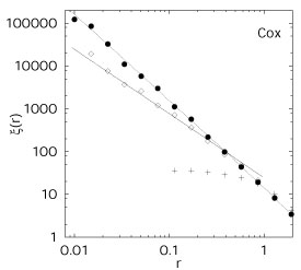
and = 10. The correlation
function estimate is shown together with the analytical
expectation of Eq. 3. Note that, at small scales,
Cox(r) ~
r- with
= 2.
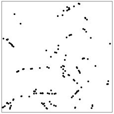
The strong clustering signal
of this point field can be smeared out by applying independent
random shifts to each point of the simulation. If the random
shifts are performed by a three-dimensional Gaussian distributed
vector with
with
= 2.
The strong clustering signal
of this point field can be smeared out by applying independent
random shifts to each point of the simulation. If the random
shifts are performed by a three-dimensional Gaussian distributed
vector with
 = 0.5, the short scale
correlations are completely
destroyed (see Fig. 4).
If the shifts are distributed according to a power-law
density probability function
d*(r)
= 0.5, the short scale
correlations are completely
destroyed (see Fig. 4).
If the shifts are distributed according to a power-law
density probability function
d*(r)
 r
r , the
value of is
reduced by 2(1 + ). In
the example
= -0.75 and therefore
changes
from 2 to 1.5. This seems to be a rather general phenomenon
[21].
The random shifts affect the correlation
function mimicking the way peculiar velocities suppress
the short range correlations
[22]
(for scales r
2h-1 Mpc, where h is the Hubble parameter in
units of 100 km s-1 Mpc-1).
, the
value of is
reduced by 2(1 + ). In
the example
= -0.75 and therefore
changes
from 2 to 1.5. This seems to be a rather general phenomenon
[21].
The random shifts affect the correlation
function mimicking the way peculiar velocities suppress
the short range correlations
[22]
(for scales r
2h-1 Mpc, where h is the Hubble parameter in
units of 100 km s-1 Mpc-1).
 |
 | |
 |
 |
 |
Figure 4. The top left panel shows a
segment Cox process simulated on a cube
with side-length 100. The top right panel shows
the two-point correlation function: The dotted line
corresponds to the expected analytical expression (see
Eq. 3), that is, in this range of scales, close to a power-law
with exponent -2. Solid bullets are the empirically calculated
values of
|
||