8.1. Large-scale magnetic fields and CMB anisotropies

Large scale magnetic fields present prior to the recombination epoch may act as a source term in the evolution equation of the cosmological perturbations. If magnetic fields are created over large length scales (possibly even larger than the Mpc) it is rather plausible that they may be present after matter-radiation equality (but before decoupling) when primordial fluctuations are imprinted on the CMB anisotropies. In fact, the relevant modes determining the large scale temperature anisotropies are the ones that are outside the horizon for _eq < < _dec where _eq and _dec are, respectively, the equality and the decoupling times. After equality there are two complementary approaches which can be used in order to address phenomenological implications of large scale magnetic fields:

• large scale magnetic fields are completely homogeneous outside the horizon after equality;

• large scale magnetic fields are inhomogeneous after equality.

The idea that homogeneous magnetic fields may affect the CMB anisotropies was originally pointed out by Zeldovich [284, 285] and further scrutinized by Grishchuk, Doroshkevich and Novikov [286]. Since this idea implies that large-scale magnetic fields are weakly gravitating the details of the discussion (and of the possible generalization of this idea) will be postponed to the following Section.

The suggestion that inhomogeneous magnetic fields created during inflation may affect the CMB anisotropies was originally proposed in [289]. In [289] it was noticed that large scale magnetic fields produced during inflation may also lead to large fluctuations for modes which are outside the horizon after equality. In [289] it was noticed that either the produced magnetic fields may be used to seed directly the CMB anisotropies, or, in a complementary persepective, the CMB data can be used to put constraints on the production mechanism.

If large-scale magnetic fields are inhomogeneous, their energy momentum tensor will have, in general terms, scalar, vector and tensor modes

(8.1)

which are decoupled and which act as source terms for the scalar, vector and tensor modes of the geometry

(8.2)

whose gauge-invariant description is well explored [199, 200] (see also [201]). The effect of the scalar component of large scale magnetic fields should be responsible, according to the suggestion of [289], of the large scale temperature anisotropies. The direct seeding of large-scale temperature anisotropies seems unlikely. In fact, the spectrum of large scale gauge fields leading to plausible values of the magnetic energy density over the scale of protogalactic collapse is typically smaller than the value required by experimental data. However, even if the primordial spectrum of magnetic fields would be tailored in an appropriate way, the initial conditions for the plasma evolution compatible with the presence of a sizable (but undercritical) magnetic field are of isocurvature type [290].

In order to illustrate this point consider the evolution equations for the gauge-invariant system of scalar perturbations of the geometry expressed in terms of the two Bardeen potential and corresponding, in the Newtonian gauge, to the fluctuations of the temporal and spatial component of the metric [200, 201]. The linearization of the (00), (0i) and (i, j) components of the Einstein equations leads, respectively, to:

(8.3) (8.4) (8.5)

where = / and w = p / is the usual barotropic index, and

(8.6)

are the fluctuations of the energy-momentum tensor of the magnetic field. Eqs. (9.10)-(8.5) have to be supplemented by the perturbation of the covariant conservation equations for the fluid sources:

(8.7) (8.8)

If the magnetic field is force-free, i.e. × × the above system simplifies. Notice that Eq. (8.8) has been already written in the case where the Lorentz force is absent. However, the forcing term appears, in the resistive MHD approximation, in Eq. (8.6). The term × × is suppressed by the conductivity, however, it can be also set exactly to zero. In this case, vector identities imply

(8.9)

i.e. _{m i} ^m = _m ^m _i. With this identity in mind the system of Eqs. (8.3)-(8.5) and (8.7)-(8.8) can be written, in Fourier space, as

(8.10) (8.11) (8.12) (8.13) (8.14)

where

(8.15)

Combining Eqs. (8.10)-(8.11) with Eq. (8.12) the following decoupled equation can be obtained

(8.16)

Consider, for simplicity, the dark-matter radiation fluid after equality and in the presence of a force-free magnetic field. In this case Eq. (8.16) can be immediately integrated:

(8.17)

The solutions given in Eq. (8.17) determine the source of the density and velocity fluctuations in the plasma, i.e.

(8.18) (8.19) (8.20) (8.21)

The solution for the velocity fields and density contrasts can be easily obtained by integrating Eqs. (8.18)-(8.21) with the source terms determined by Eq. (8.17). The purpose is not to integrate here this system (see for instance [291] for the standard case without magnetic fields). Rather it is important to notice that there are two qualitatively different situation. The first situation is the one where,

(8.22)

namely the case where the constant mode of the Bardeen potential is negligible if compared to the contribution of the magnetic field. The derivative of the Bardeen potential will be, however, non vanishing. In this case the CMB anisotropies are said to be seeded by isocurvature initial conditions for the fluid of radiation and dark-matter present after equality. In the opposite case, nemely

(8.23)

the constant mode of the Bardeen potential is provided, for instance, by inflation and the magnetic field represent a further parameter to be taken into account in the analysis of CMB anisotropies. Assuming, roughly, that |₀(k)| ~ 10^-6, Eq. (8.23) implies that for the typical scale of the horizon at decoupling the critical fraction of magnetic energy density should be smaller than 10^-3. In the case of Eq. (8.23) the leading order relations among the different hydrodynamical fluctuations are well known and can be obtained from Eqs. (8.18)-(8.21) if the magnetic field is approximately negligible, i.e.

(8.24)

This result has a simple physical interpretation, and implies the adiabaticity of the fluid perturbations. The entropy per matter particle is indeed proportional to S = T³ / n_m, where n_m is the number density of matter particles and T is the radiation temperature. The associated entropy fluctuation, S, satisfies

(8.25)

where we used the fact that _r ~ T⁴ and that _m = mn_m, where m is the typical mass of the particles in the matter fluid. Equation (8.24) thus implies S / S = 0, in agreement with the adiabaticity of the fluctuations.

After having computed the corrections induced by the magnetic field on the (leading) adiabatic initial condition the temperature anisotropies can be computed using the Sachs-Wolfe effect [292]. In terms of the gauge-invariant variables introduced in the present analysis, the various contributions to the Sachs-Wolfe effect, along the direction, can be written as

(8.26)

where ₀ is the present time, and () = ₀ - ( - ₀) is the unperturbed photon position at the time for an observer in ₀. The term _b is the peculiar velocity of the baryonic matter component.

In Fig. 11 the C are plotted in the case of models with adiabatic initial conditions.

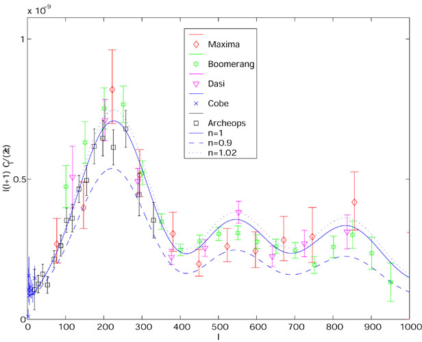Figure 11. The spectrum of C is illustrated for a fiducial set of parameters (h0 = 0.65, b = 0.04733, = 0.7, m = 0.25267) and for flat (full line, n = 1), slightly red (dashed line, n = 0.9) and slightly blue (dotted line, n = 1.02) spectral indices for the constant (adiabatic) mode.

The data points reported in Figs. 11 and 12 are those from COBE [293, 294], BOOMERANG [295], DASI [296], MAXIMA [297] and ARCHEOPS [298]. Notice that the data reported in [298] fill the "gap" between the last COBE points and the points of [295, 296, 297]. In Fig. 12 the recent WMAP data are reported [299, 300, 301].

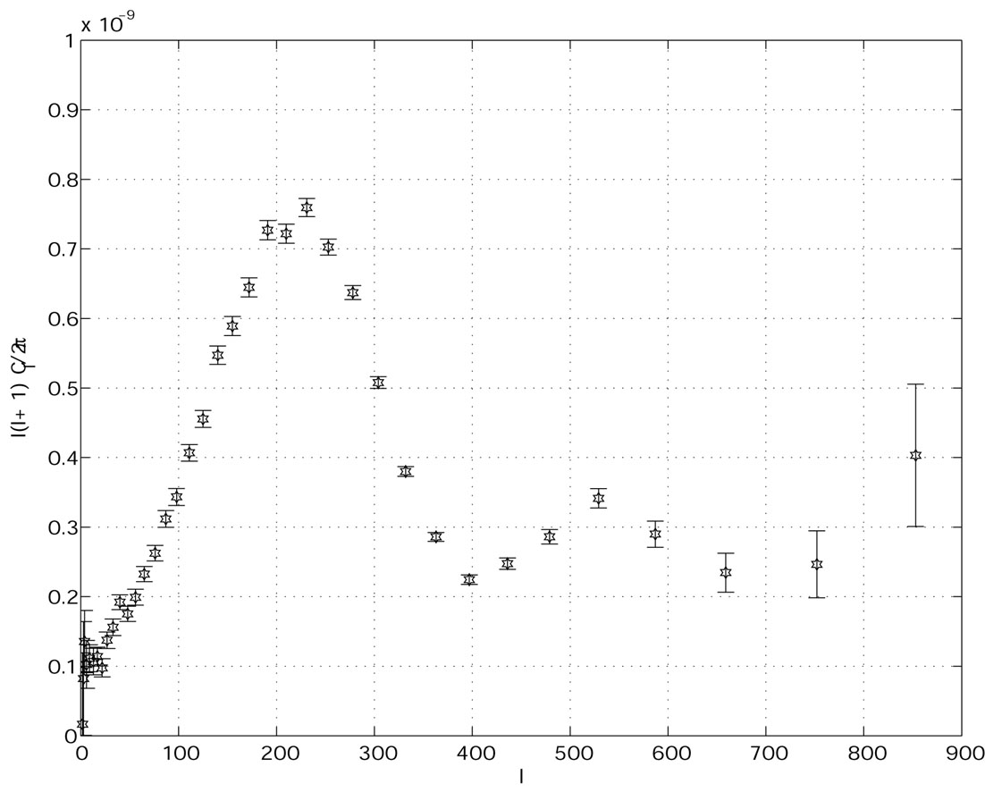Figure 12. The WMAP data are reported.

Recall, that the temperature fluctuations are customarily discussed in terms of their Legendre transform

(8.27)

where the coefficients a_m define the angular power spectrum C by

(8.28)

and determine the two-point (scalar) correlation function of the temperature fluctuations, namely

(8.29)

In Fig. 11 and 12 the experimental points are presented in terms of the C spectra.

In Fig. 11 and 12 the curves fitting the data are obtained by imposing adiabatic initial conditions. If magnetic fields would seed directly the CMB anisotropies a characteristic "hump" would appear for < 100 which is not compatible with the experimental data. If, on the contrary, the condition (8.23) holds, then the modifications due to a magnetic field can be numerically computed for a given magnetic spectral index and for a given amplitude. This analysis has been performed by Koh and Lee [302]. The claim is that by modifying the amplitude of the magnetic field in a way compatible with the cosmological constraint the effect on the scalar C can be as large as the 10% for a given magnetic spectral index.

The main problem is order to detect large-scale magnetic fields from the spectrum of temperature fluctuations is the parameter space. On top of the usual parameters common in the CMB analysis at least two new parameters should be introduced, namely the magnetic spectral index and the amplitude of the magnetic field. The proof of this statement is that there is no available analysis of the WMAP data including also the presence of large scale magnetic fields in the initial conditions according to the lines presented in this Section.

To set bounds on primordial magnetic fields from CMB anisotropies it is often assumed that the magnetic field is fully homogeneous. In this case the magnetic field amplitude has been bounded to be B 10^-3 G at the decoupling time [303] (see also [305] for a complementary analysis always in the case of a homogeneous magnetic field).

There is the hope that since magnetic fields contribute not only to the scalar fluctuations, but also to the vector and tensor modes of the geometry useful informations cann be also obtained from the analysis of vector and tensor power spectra. In [304] temperature and polarization power spectra induced by vector and tensor perturbations have been computed by assuning a power-law spectrum of magnetic inhomogeneities. In [306, 307, 308] the tensor modes of the geometry have been specifically investigated. In [309, 310, 311] it is argued that magnetic fields can induce anisotropies in the polarization for rather small length scales, i.e. > 1000.

As already pointed out in the present Section, magnetic fields may be assumed to be force free in various cases. This is an approximation which may also be relaxed. However, even if magnetic fields are assumed to be force-free there is no reason to assume that their associated magnetic helicity (or gyrotropy) vanishes. In [312] the posssible effects of helical magnetic fields on CMB physics have been investigated. If helical flows are present at recombination, they would produce parity violating temperature-polarization correlations. The magnitude of helical flows induced by helical magnetic fields turns out to be unobservably small, but better prospects of constraining helical magnetic fields come from maps of Faraday rotation measurements of the CMB [312].