3.3. N-body models

The exact evolution of the density field is usually performed by means of an N-body simulation, in which the density field is represented by the sum of a set of fictitious discrete particles. The equations of motion for each particle depend on solving for the gravitational field due to all the other particles, finding the change in particle positions and velocities over some small time step, moving and accelerating the particles, and finally re-calculating the gravitational field to start a new iteration. Using comoving units for length and velocity (v = a u), we have previously seen the equation of motion

(64)

where is the Newtonian gravitational potential due to density perturbations. The time derivative is already in the required form of the convective time derivative observed by a particle, rather than the partial / t. If we change time variable from t to a, this becomes

(65)

Here, the gravitational acceleration has been written exactly by summing over all particles, but this becomes prohibitive for very large numbers of particles. Since the problem is to solve Poisson's equation, a faster approach is to use Fourier methods, since this allows the use of the fast Fourier transform (FFT) algorithm (see chapter 13 of Press et al. 1992). If the density perturbation field (not assumed small) is expressed as = _k exp(- ik ^. x), then Poisson's equation becomes - k² _k = 4 Ga² _k, and the required k-space components of are just

(66)

If we finally eliminate matter density in terms of _m, the equation of motion for a given particle is

(67)

This can be expressed more neatly by defining dimensionless units that incorporate the the side of the box, L:

(68)

For N particles, the density is = Nm / (aL)³, so the mass of the particles and the gravitational constant can be eliminated and the equation of motion can be cast in an attractively dimensionless form:

(69)

The function f (a) is proportional to a²H(a), and has an arbitrary normalization - e.g. unity at the initial epoch.

Particles are now moved according to dx = u dt, which becomes

(70)

It only remains to set up the initial conditions; this is easy to do if the initial epoch is at high enough redshift that _m = 1, since then U a and the earlier discussion of Lagrangian perturbations shows that velocities and the initial displacements are related by

(71)

The simplest N-body algorithm for solving the equations of motion is the particle-mesh (PM) code. This averages the density field onto a grid and uses the FFT algorithm both to perform the transformation of density and to perform the (three) inverse transforms to obtain the real-space force components from their k-space counterparts (see Hockney & Eastwood 1988; Efstathiou et al. 1985). The resolution of a PM code is clearly limited to about the size of the mesh. To do better, one can use a particle-particle-particle-mesh (PM) code, also discussed by the above authors. Here, the direct forces are evaluated between particles in the nearby cells, with the grid estimate being used only for particles in more distant cells. An alternative approach is to use adaptive mesh codes, in which high-density regions are re-gridded to use a finer mesh (e.g. Kravtsov, Klypin & Khokhlov 1997). A similar effect, although without the use of a mesh, is achieved by tree codes (e.g. Hernquist, Bouchet & Suto 1991).

In practice, however, the increase in resolution gained from these methods is limited to a factor of 10. This is because each particle in a cosmological N-body simulation in fact stands for a large number of less massive particles. Close encounters of these spuriously large particles can lead to wide-angle scattering, whereas the true physical systems are completely collisionless. To prevent collisions, the forces must be softened, i.e. set to a constant below some critical separation, rather than rising as 1/r². If there are already few particles per PM cell, the softening must be some significant fraction of the cell size, so there is a limit to the gain over pure PM.

Despite these caveats, the results of N-body dynamics paint an impressive picture of the large-scale mass distribution. Consider figure 3, which shows slices through the computational density field for two particular sets of initial conditions, with different relative amplitudes of long and short wavelengths, but with the same amplitude for the modes with wavelengths equal to the side of the computational box. Although the small-scale `lumpiness' is different, both display a similar large-scale network of filaments and voids - bearing a striking resemblance to the features seen in reality.

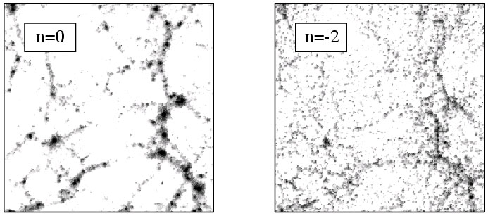Figure 3. Slices through N-body simulations of different power spectra, using the same set of random phases for the modes in both cases. The slices are 1/15 of the box in thickness, and density from 0.5 to 50 is log encoded. The box-scale power is the same in both cases, and produces much the same large-scale filamentary structure. However, the n = 0 spectrum has much more small-scale power, and this manifests itself as far stronger clumping within the overall skeleton of the structure.

The state of the art in these calculations now routinely involves 10⁸ to 10⁹ particles, covering box sizes from the minimum necessary so that the box-scale modes do not saturate (~ 100 h^-1 Mpc) to effectively the entire observable universe (e.g. Evrard et al. 2002). The resolution available in the smaller boxes is sufficient that the nonlinear evolution of collisionless mass distributions is now effectively a solved problem, and nonlinear clustering statistics for model universes of practical interest can be measured to a few % precision (e.g. Jenkins et al. 1998). Further improvements in these sort of calculations are unlikely to be of practical importance, because of the need to include the evolution of the baryonic component, which makes up around 20% of the total matter density. The history of the gas is immensely complex, since it is strongly influenced by feedback of energy from the stars that form within it. The limitation of our modelling of such processes lies not so much in simple numerical aspects such as resolution, but in the simplifying assumptions used to treat processes that occur on scales very far below the resolution of any simulation. See e.g. Katz, Weinberg & Hernquist (1996); Pearce et al. (2001).